2.2 Reproducing kernels and transformation maps

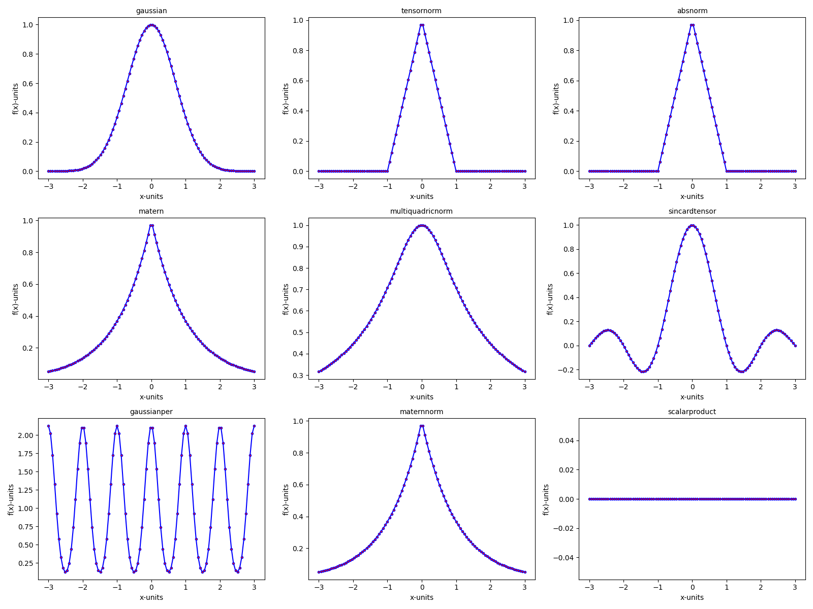
In this experiment, we plot in 2D and 3D various kernels available in CodPy.

# Importing necessary modules
import os
import sys

curr_f = os.path.join(os.getcwd(), "codpy-book", "utils")
sys.path.insert(0, curr_f)


import matplotlib.pyplot as plt
import numpy as np

# import CodPy's core module and Kernel class
from codpy import core
from codpy.kernel import Kernel

# from codpy.plotting import plot1D
# Lets import multi_plot function from codpy utils
from codpy.plot_utils import multi_plot, plot1D


def kernel_fun(x=None, kernel_name=None, D=1):
    if x is None:
        x = np.linspace(-3, 3, num=100)
    y = np.zeros([1, D])
    kernel = Kernel(
        set_kernel=core.kernel_setter(kernel_name, None),
        x=x,
        order=1,
    )
    out = kernel.knm(x, y)
    return out


def kernel_funs_plot():
    kernel_list = [
        "gaussian",
        "tensornorm",
        "absnorm",
        "matern",
        "multiquadricnorm",
        # "multiquadrictensor",
        "sincardtensor",
        # "sincardsquaretensor",
        # "dotproduct",
        "gaussianper",
        "maternnorm",
        "scalarproduct",
    ]

    # Prepare the results for plotting each kernel
    results = [
        (np.linspace(-3, 3, num=100), kernel_fun(kernel_name=kernel_name).flatten())
        for kernel_name in kernel_list
    ]

    # Legends for each kernel in the plot
    legends = kernel_list

    # Plot all kernels using multi_plot in a 4x4 grid
    multi_plot(
        results,
        plot1D,
        f_names=legends,
        mp_nrows=3,
        mp_ncols=3,
        mp_figsize=(16, 12),
    )


# Run the experiment with CodPy and SciPy models
# core.KerInterface.set_verbose()
kernel_funs_plot()
plt.show()

Kernel Gram matrix Positive definite kernels and kernel matrices. A kernel, denoted by \(k: \mathbb{R}^D \times \mathbb{R}^D \to \mathbb{R}\), is a symmetric real-valued function, that is, satisfying \(k(x, y)=k(y, x)\). Given two collections of points in \(\mathbb{R}^D\), namely \(X = (x^1, \cdots, x^{N_x})\) and \(Y = (y^1, \cdots, y^{N_y})\), we define the associated kernel matrix \(K(X,Y) = \big(k(x^n,y^m) \big) \in \mathbb{R}^{N_x, N_y}\) by

\[\begin{split}K(X, Y) =\left( \begin{array}{ccc} k(x^1,y^1) & \cdots & k(x^1,y^{N_y}) \\ \ddots & \ddots & \ddots \\ k(x^{N_x},y^1) & \cdots & k(x^{N_x},y^{N_y}) \end{array}\right).\end{split}\]

import pandas as pd

x = np.random.randn(10, 1)
kernel = Kernel(
    set_kernel=core.kernel_setter("gaussian", None),
    x=x,
    order=1,
)

# Kernel Gram matrix
print(pd.DataFrame(kernel.knm(x, x)))

          0         1         2         3         4         5         6         7         8         9
0  1.000000  0.039997  0.485097  0.001687  0.969665  0.163022  0.626316  0.810604  0.881845  0.746901
1  0.039997  1.000000  0.000917  0.584600  0.020660  0.818636  0.291607  0.167854  0.009882  0.207555
2  0.485097  0.000917  1.000000  0.000011  0.634033  0.008000  0.094904  0.180349  0.781960  0.144546
3  0.001687  0.584600  0.000011  1.000000  0.000674  0.248462  0.033511  0.013855  0.000248  0.019319
4  0.969665  0.020660  0.634033  0.000674  1.000000  0.098526  0.477680  0.669228  0.968437  0.599145
5  0.163022  0.818636  0.008000  0.248462  0.098526  1.000000  0.644512  0.454047  0.055313  0.521736
6  0.626316  0.291607  0.094904  0.033511  0.477680  0.644512  1.000000  0.950292  0.340020  0.979527
7  0.810604  0.167854  0.180349  0.013855  0.669228  0.454047  0.950292  1.000000  0.516495  0.993303
8  0.881845  0.009882  0.781960  0.000248  0.968437  0.055313  0.340020  0.516495  1.000000  0.449026
9  0.746901  0.207555  0.144546  0.019319  0.599145  0.521736  0.979527  0.993303  0.449026  1.000000

MMD Matrix

MMD matrices provide a very useful tool in order to evaluate the accuracy of a computation. To any positive kernel \(k : \mathbb{R}^D, \mathbb{R}^D \mapsto \mathbb{R}\), we associate the discrepancy function \(d_k(x,y)\) defined (for \(x,y\in\mathbb{R}^D\)) by

\[d_k(x,y) = k(x,x) + k(y,y) - 2k(x,y)\]

. For positive kernels, \(d_k(\cdot,\cdot)\) is continuous, non-negative, and satisfies the condition \(d_k(x,x) = 0\) (for all relevant \(x\))

print(pd.DataFrame(kernel.kernel_distance(x)))

          0         1         2         3         4         5         6         7         8         9
0  0.000000  1.920006  1.029805  1.996626  0.060669  1.673956  0.747368  0.378793  0.236310  0.506198
1  1.920006  0.000000  1.998166  0.830799  1.958679  0.362728  1.416785  1.664292  1.980237  1.584890
2  1.029805  1.998166  0.000000  1.999978  0.731933  1.983999  1.810192  1.639303  0.436080  1.710907
3  1.996626  0.830799  1.999978  0.000000  1.998652  1.503076  1.932979  1.972290  1.999504  1.961362
4  0.060669  1.958679  0.731933  1.998652  0.000000  1.802948  1.044641  0.661543  0.063126  0.801710
5  1.673956  0.362728  1.983999  1.503076  1.802948  0.000000  0.710976  1.091906  1.889375  0.956529
6  0.747368  1.416785  1.810192  1.932979  1.044641  0.710976  0.000000  0.099416  1.319960  0.040947
7  0.378793  1.664292  1.639303  1.972290  0.661543  1.091906  0.099416  0.000000  0.967011  0.013395
8  0.236310  1.980237  0.436080  1.999504  0.063126  1.889375  1.319960  0.967011  0.000000  1.101947
9  0.506198  1.584890  1.710907  1.961362  0.801710  0.956529  0.040947  0.013395  1.101947  0.000000

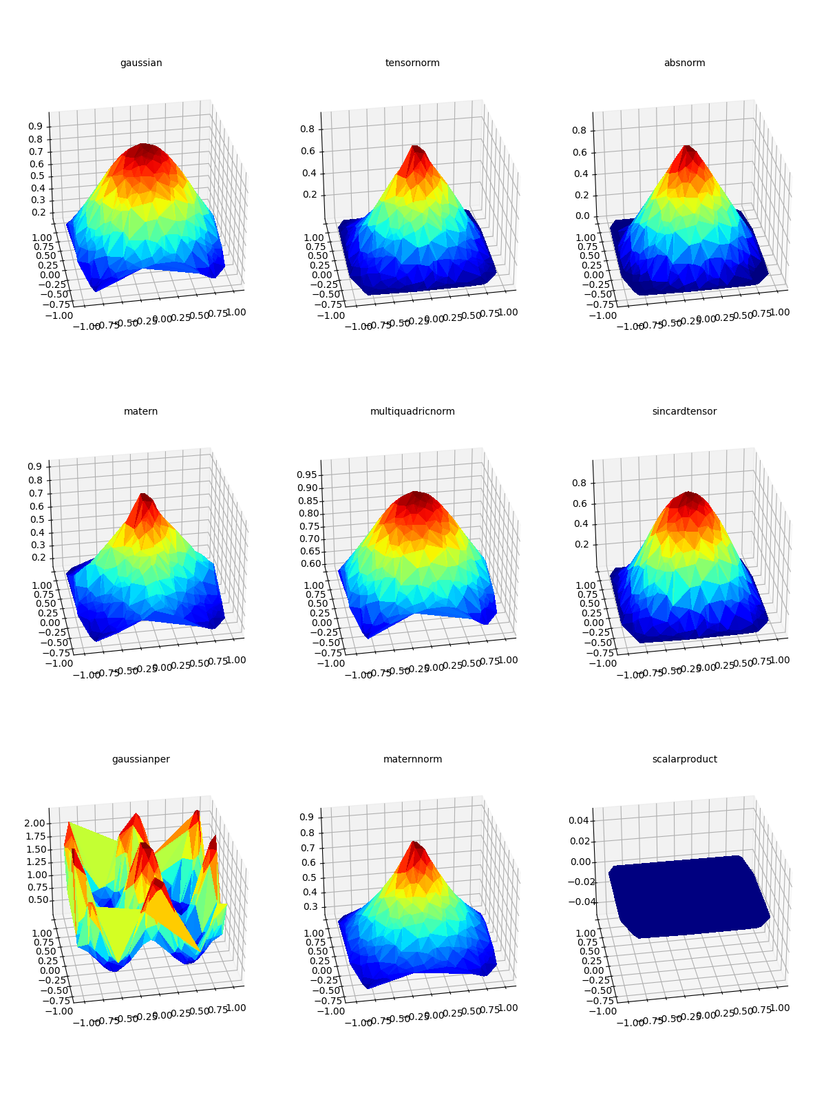
Kernels 2D visualisation

# Lets define helper function to plot 3D projection of the function
def plot_trisurf(xfx, ax, legend="", elev=90, azim=-100, **kwargs):
    from matplotlib import cm

    """
    Helper function to plot a 3D surface using a trisurf plot.

    Parameters:
    - xfx: A tuple containing the x-coordinates (2D points) and their
      corresponding function values.
    - ax: The matplotlib axis object for plotting.
    - legend: The legend/title for the plot.
    - elev, azim: Elevation and azimuth angles for the 3D view.
    - kwargs: Additional keyword arguments for further customization.

    """

    xp, fxp = xfx[0], xfx[1]
    x, fx = xp, fxp

    X, Y = x[:, 0], x[:, 1]
    Z = fx.flatten()
    ax.plot_trisurf(X, Y, Z, antialiased=False, cmap=cm.jet)
    ax.view_init(azim=azim, elev=elev)
    ax.title.set_text(legend)


def generate2Ddata(sizes_x):
    data_x = np.random.uniform(-1, 1, (sizes_x, 2))

    kernel_list = [
        "gaussian",
        "tensornorm",
        "absnorm",
        "matern",
        "multiquadricnorm",
        # "multiquadrictensor",
        "sincardtensor",
        # "sincardsquaretensor",
        # "dotproduct",
        "gaussianper",
        "maternnorm",
        "scalarproduct",
    ]

    # Prepare the results for plotting each kernel
    results = [
        (data_x, kernel_fun(data_x, kernel_name, D=2).flatten())
        for kernel_name in kernel_list
    ]

    # Legends for each kernel in the plot
    legends = kernel_list

    # Plot all kernels using multi_plot in a 4x4 grid
    multi_plot(
        results,
        plot_trisurf,
        f_names=legends,
        mp_nrows=3,
        mp_ncols=3,
        mp_figsize=(12, 16),
        elev=30,
        projection="3d",
    )


generate2Ddata(400)
plt.show()
pass