2.4 2D Periodic Function Extrapolation

This script demonstrates an experiment using CodPy and SciPy models to visualize a 2D periodic function. It generates random data points (x, fx) and (z, fz), applies both CodPy and SciPy models, and visualizes the results using 3D plots.

The script is divided into several parts:

• Data generation: Creating random periodic data for different sizes.

• Plotting: Inline plotting of generated and modeled data.

• Model application: Applying CodPy and SciPy models for interpolation.

# Importing necessary modules
import os
import sys
import time

curr_f = os.path.join(os.getcwd(), "codpy-book", "utils")
sys.path.insert(0, curr_f)


import matplotlib.pyplot as plt
import numpy as np
from scipy.interpolate import Rbf

# import CodPy's core module and Kernel class
from codpy import core
from codpy.kernel import Kernel

# from codpy.plotting import plot1D
# Lets import multi_plot function from codpy utils
from codpy.plot_utils import multi_plot

from sklearn.metrics import mean_squared_error

# Define the sinusoidal function
def periodic_fun(x):
    """
    A sinusoidal function that generates a sum of sines based on the input ``x``.
    """
    from math import pi

    sinss = np.cos(2 * x * pi)
    if x.ndim == 1:
        sinss = np.prod(sinss, axis=0)
        ress = np.sum(x, axis=0)
    else:
        sinss = np.prod(sinss, axis=1)
        ress = np.sum(x, axis=1)
    return ress + sinss


# Lets define helper function to plot 3D projection of the function
def plot_trisurf(xfx, ax, legend="", elev=90, azim=-100, **kwargs):
    from matplotlib import cm

    """
    Helper function to plot a 3D surface using a trisurf plot.

    Parameters:
    - xfx: A tuple containing the x-coordinates (2D points) and their
      corresponding function values.
    - ax: The matplotlib axis object for plotting.
    - legend: The legend/title for the plot.
    - elev, azim: Elevation and azimuth angles for the 3D view.
    - kwargs: Additional keyword arguments for further customization.
    """

    xp, fxp = xfx[0], xfx[1]
    x, fx = xp, fxp

    X, Y = x[:, 0], x[:, 1]
    Z = fx.flatten()
    ax.plot_trisurf(X, Y, Z, antialiased=False, cmap=cm.jet)
    ax.view_init(azim=azim, elev=elev)
    ax.title.set_text(legend)


# Function to generate periodic data
def generate_periodic_data(sizes_x, sizes_z):
    """
    Generates 2D periodic data for given sizes of x and z.

    Parameters:
    - sizes_x: List of sizes for the x data.
    - sizes_z: List of sizes for the z data.

    Returns:
    - data_x: List of generated x arrays.
    - data_fx: List of function values corresponding to each x.
    - data_z: List of generated z arrays.
    - data_fz: List of function values corresponding to each z.
    """
    # Generate x and z data of different sizes
    data_x = [np.random.uniform(-1, 1, (size, 2)) for size in sizes_x]
    data_z = [np.random.uniform(-1.5, 1.5, (size, 2)) for size in sizes_z]

    # Compute fx for each x and fz for each z
    data_fx = [periodic_fun(x).reshape(-1, 1) for x in data_x]
    data_fz = [periodic_fun(z).reshape(-1, 1) for z in data_z]

    return data_x, data_fx, data_z, data_fz


# Function to plot the generated data points
def plot_x_fx_z_fz(N=1024):
    """
    Inline plot of the periodic data (x, fx) and (z, fz) for a fixed size N.

    Parameters:
    - N: Size of the generated x and z arrays (default is 1024).
    """
    # Generate x and z data of size N
    x = np.random.uniform(-1, 1, (N, 2))
    z = np.random.uniform(-1.5, 1.5, (N, 2))

    # Compute fx for x and fz for z
    fx = periodic_fun(x).reshape(-1, 1)
    fz = periodic_fun(z).reshape(-1, 1)

    # Prepare the results for plotting (x, fx) and (z, fz) pairs
    results = [(x, fx), (z, fz)]

    # Legends for the subplots, displaying the size of x and z
    legends = [f"Data (x, fx) with N = {N}", f"Data (z, fz) with N = {N}"]

    # Plot the data using multi_plot in a 1x2 grid
    multi_plot(
        results,
        plot_trisurf,
        mp_nrows=1,
        mp_ncols=2,
        mp_figsize=(12, 6),
        legends=legends,
        projection="3d",
    )


# lets output the plot
plot_x_fx_z_fz()

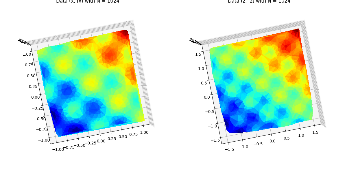
The plot shows a sinusoidal pattern for the data generated in the cartesian coordinate system. The two curves for x and z exhibits the sinusoidal variations defined by periodic_fun(x).

Model Setup and Training

---

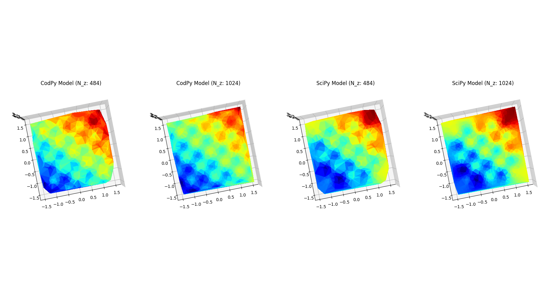
def run_experiment(data_x, data_fx, data_z):
    """
    Runs the experiment applying CodPy and SciPy models on the data and plots the results.

    Parameters:
    - data_x: List of generated x arrays.
    - data_fx: List of function values corresponding to each x.
    - data_z: List of generated z arrays.
    """
    # Apply CodPy and SciPy models for each (x, fx, z) pair
    codpy_models = [(z, codpy_model(x, fx, z)) for x, fx, z in zip(data_x, data_fx, data_z)]

    mmds_res = [np.sqrt(model.discrepancy(z)) for z, model in codpy_models] + \
        [None for z in data_z]
    model_results = [
        (z, cp_model(z)) for x, fx, z, (_,cp_model) in zip(data_x, data_fx, data_z, codpy_models)
    ] + [(z, rbf_interpolator(x, fx, z)) for x, fx, z in zip(data_x, data_fx, data_z)]

    # Titles for each subplot
    legends = [f"CodPy Model (N_z: {z.shape[0]})" for z in data_z] + [
        f"SciPy Model (N_z: {z.shape[0]})" for z in data_z
    ]

    # Plot the model results using multi_plot
    multi_plot(
        model_results,
        plot_trisurf,
        mp_nrows=1,
        mp_ncols=4,
        mp_figsize=(18, 10),
        legends=legends,
        projection="3d",
    )

    model_functions = [codpy_pred, rbf_interpolator]
    Nxs = [x.shape[0] for x in data_x]
    results = {}
    times = {}
    mmds = {}
    for j, Nx in enumerate(Nxs):
        results[Nx] = {}
        times[Nx] = {}
        mmds [Nx] = {}
        for i, model in enumerate(model_functions):
            start = time.perf_counter()
            _, f_z = model_results[j if i == 0 else j + len(data_x)]
            mmd = mmds_res[j if i == 0 else j + len(data_x)]
            end = time.perf_counter()
            mmds[Nx][model.__name__] = mmd
            results[Nx][model.__name__] = mean_squared_error(data_fz[j], f_z)
            times[Nx][model.__name__] = end - start
            print(f"Model: {model.__name__}, Time taken: {end-start:.4f} seconds")

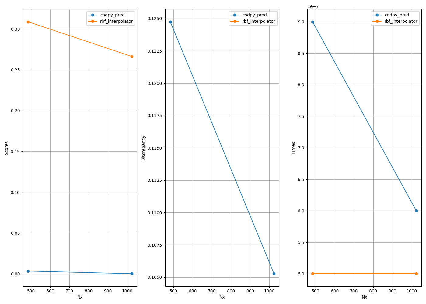
    res = [{"data": results}, {"data": mmds}, {"data": times}]

    def plot_one(inputs):
        results = inputs["data"]
        ax = inputs["ax"]
        legend = inputs["legend"]
        for model_name in next(iter(results.values())).keys():
            x_vals = sorted(results.keys())
            y_vals = [results[x][model_name] for x in x_vals]
            ax.plot(x_vals, y_vals, marker='o', label=model_name)
        ax.set_xlabel('Nx')
        ax.set_ylabel(legend)
        ax.legend()
        ax.grid(True)

    multi_plot(
        res,
        plot_one,
        mp_nrows=1,
        mp_ncols=3,
        legends=["Scores", "Discrepancy", "Times"],
        mp_figsize=(14, 10),
    )
    plt.show()

# Applies CodPy's kernel-based model for interpolation.
def codpy_model(x, fx, z):
    kernel = Kernel(
        set_kernel=core.kernel_setter("gaussianper", None,2,1e-9),
        x=x,
        fx=fx,
        order=2,
    )
    return kernel

def codpy_pred(x,fx,z):
    return codpy_model(x, fx, z)(z)

# SciPy RBF Interpolator for 2D data interpolation.
def rbf_interpolator(x, fx, z):
    """
    SciPy RBF Interpolator for 2D data interpolation.

    Parameters:
    - x: A (N, 2) array of 2D coordinates.
    - fx: A (N, 1) array of corresponding function values.
    - z: A (M, 2) array of new coordinates where we want to interpolate.

    Returns:
    - Interpolated function values at points in z.
    """
    # Split the 2D x array into separate arrays for each dimension
    x1, x2 = x[:, 0], x[:, 1]

    # Flatten fx to be a 1D array
    fx_flat = fx.ravel()

    # Create the Rbf interpolator using the separate dimensions of x
    rbf = Rbf(x1, x2, fx_flat, function="multiquadric")

    # Split the 2D z array into separate arrays for each dimension
    z1, z2 = z[:, 0], z[:, 1]

    # Return the interpolated values at points in z
    return rbf(z1, z2).reshape(-1, 1)


# Example Usage
sizes_x = [484, 1024]
sizes_z = [484, 1024]

# Generate the data
data_x, data_fx, data_z, data_fz = generate_periodic_data(sizes_x, sizes_z)

# Run the experiment with CodPy and SciPy models
run_experiment(data_x, data_fx, data_z)
plt.show()
pass

• 
• 

Model: codpy_pred, Time taken: 0.0000 seconds
Model: rbf_interpolator, Time taken: 0.0000 seconds
Model: codpy_pred, Time taken: 0.0000 seconds
Model: rbf_interpolator, Time taken: 0.0000 seconds