Note
Go to the end to download the full example code.
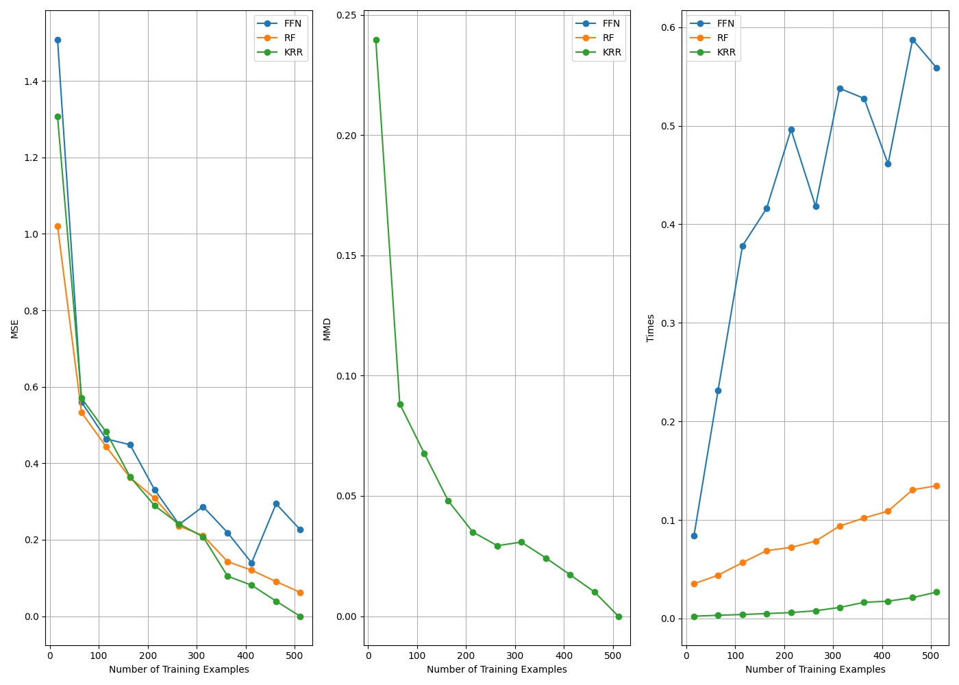
6.1 Supervised learning: reproducibility illustration with housing prices
We show how to reproduce the results of the chapter 6.2.1 - Application to supervised machine learning - Regression problem: housing price prediction of the book. We will compare the codpy model with other standard regression methods. The goal is to show the codpy model capacity to fit the training data.
- Necessary Imports
import sys
import os
import time
from pathlib import Path

try:
    base_path = Path(__file__).parent.parent
except NameError:
    base_path = Path.cwd().parent

sys.path.append(str(base_path))

try:
    CURRENT_DIR = os.path.dirname(os.path.abspath(__file__))
except NameError:
    CURRENT_DIR = os.getcwd()
data_path = os.path.join(CURRENT_DIR, "data")
PARENT_DIR = os.path.abspath(os.path.join(CURRENT_DIR, ".."))
sys.path.insert(0, PARENT_DIR)

import matplotlib.pyplot as plt
import numpy as np
import torch
import torch.nn as nn
from utils.ch9.path_generation import California_data_generator
from sklearn.ensemble import RandomForestRegressor
from sklearn.preprocessing import StandardScaler

from codpy.kernel import Kernel
from codpy.plot_utils import multi_plot
Regression models
In the following methods we define the regression models to be used for the comparison. Each model gets evaluated on the training data based on the Mean Squared Error (MSE) loss. We also compute the Maximum Mean Discrepancy (MMD) for the codpy model, used to showcase the direct inverse relationship between MMD and Score.
To use CodPy for regression, we instanciate a Kernel object and pass x as the training data and fx as the target values. Calling the kernel with z will return the predictions, similar to how we would use predict().
def codpy_model(x, fx, z, fz):
    kernel = Kernel(
        x=x,
        fx=fx,
    )
    results = kernel(z)
    eval_loss = np.mean((results - fz) ** 2)
    mmd = np.sqrt(kernel.discrepancy(z))
    return eval_loss, mmd


# Different other standard models are defined below.
# The user can add these models to the lists of models to be evaluated.
def torch_model(x, fx, z, fz):
    input_scaler = StandardScaler()
    x = input_scaler.fit_transform(x)
    z = input_scaler.transform(z)

    target_scaler = StandardScaler()
    fx = target_scaler.fit_transform(fx.reshape(-1, 1)).reshape(-1)
    fz_scaled = target_scaler.transform(fz.reshape(-1, 1)).reshape(-1)

    x = torch.tensor(x, dtype=torch.float32)
    fx = torch.tensor(fx, dtype=torch.float32)
    z = torch.tensor(z, dtype=torch.float32)
    fz = torch.tensor(fz_scaled, dtype=torch.float32)

    class FFN(nn.Module):
        def __init__(self, input_dim):
            super().__init__()
            self.net = nn.Sequential(
                nn.Linear(input_dim, 64),
                nn.ReLU(),
                nn.Linear(64, 128),
                nn.ReLU(),
                nn.Linear(128, 64),
                nn.ReLU(),
                nn.Linear(64, 1),
            )

        def forward(self, x):
            return self.net(x)

    model = FFN(x.shape[1])
    optimizer = torch.optim.AdamW(model.parameters(), lr=0.001, weight_decay=1e-3)
    loss_fn = nn.MSELoss()

    n_samples = x.shape[0]
    batch_size = max(n_samples // 4, 32)

    start_time = time.perf_counter()

    model.train()
    for epoch in range(128):
        indices = torch.randperm(n_samples)
        for start in range(0, n_samples, batch_size):
            end = min(start + batch_size, n_samples)
            batch_idx = indices[start:end]
            x_batch = x[batch_idx]
            fx_batch = fx[batch_idx]

            pred = model(x_batch).squeeze()
            loss = loss_fn(pred, fx_batch)

            optimizer.zero_grad()
            loss.backward()
            optimizer.step()

    model.eval()
    with torch.no_grad():
        pred_scaled = model(z).squeeze().numpy()
        pred = target_scaler.inverse_transform(pred_scaled.reshape(-1, 1)).reshape(-1)
        true = target_scaler.inverse_transform(fz.numpy().reshape(-1, 1)).reshape(-1)
        eval_loss = np.mean((pred - true) ** 2)

    return eval_loss, None


def random_forest_model(x, fx, z, fz):
    x, fx, z, fz = np.array(x), np.array(fx).ravel(), np.array(z), np.array(fz).ravel()
    model = RandomForestRegressor(n_estimators=100, random_state=42)
    model.fit(x, fx)
    results = model.predict(z)
    eval_loss = np.mean((results - fz) ** 2)
    return eval_loss, None


def adaboost_model(x, fx, z, fz):
    x, fx, z, fz = np.array(x), np.array(fx).ravel(), np.array(z), np.array(fz).ravel()
    from sklearn.ensemble import AdaBoostRegressor

    model = AdaBoostRegressor(n_estimators=50, learning_rate=1)
    model.fit(x, fx)
    results = model.predict(z)
    eval_loss = np.mean((results - fz) ** 2)
    return eval_loss, None


def xgboost_model(x, fx, z, fz):
    x, fx, z, fz = np.array(x), np.array(fx).ravel(), np.array(z), np.array(fz).ravel()
    import xgboost as xgb

    model = xgb.XGBRegressor(n_estimators=100, learning_rate=0.1)
    model.fit(x, fx)
    results = model.predict(z)
    eval_loss = np.mean((results - fz) ** 2)
    return eval_loss, None


def svr_model(x, fx, z, fz):
    x, fx, z, fz = np.array(x), np.array(fx).ravel(), np.array(z), np.array(fz).ravel()
    from sklearn.svm import SVR

    model = SVR(kernel="rbf", C=1.0, epsilon=0.1)
    model.fit(x, fx)
    results = model.predict(z)
    eval_loss = np.mean((results - fz) ** 2)
    return eval_loss, None


def gradient_boosting_model(x, fx, z, fz):
    x, fx, z, fz = np.array(x), np.array(fx).ravel(), np.array(z), np.array(fz).ravel()
    from sklearn.ensemble import GradientBoostingRegressor

    model = GradientBoostingRegressor(n_estimators=100, learning_rate=0.1)
    model.fit(x, fx)
    results = model.predict(z)
    eval_loss = np.mean((results - fz) ** 2)
    return eval_loss, None


def decision_tree_model(x, fx, z, fz):
    x, fx, z, fz = np.array(x), np.array(fx).ravel(), np.array(z), np.array(fz).ravel()
    from sklearn.tree import DecisionTreeRegressor

    model = DecisionTreeRegressor(max_depth=5)
    model.fit(x, fx)
    results = model.predict(z)
    eval_loss = np.mean((results - fz) ** 2)
    return eval_loss, None
Gathering Results
Here we benchmark 3 of the models defined above. We use the California housing dataset, and train the models on different subsets of the training dataset. We always evaluate the models on the entire training set. Therefore, the last training procedure trains and evaluate on the exact same data.
results = {}
times = {}
mmds = {}
models = [torch_model, random_forest_model, codpy_model]
model_aliases = {
    "torch_model": "FFN",
    "codpy_model": "KRR",
    "random_forest_model": "RF",
}
data_generator_ = California_data_generator()
X, FX, X, FX, Z, FZ = data_generator_.get_data(-1, -1, -1, -1)
torch.manual_seed(0)
idxs = torch.randperm(len(X))
SIZE = 512
X, FX, Z, FZ = (
    X.values[idxs][:SIZE],
    FX.values[idxs][:SIZE],
    Z.values[idxs][:SIZE],
    FZ.values[idxs][:SIZE],
)
length_ = len(X)
# Different slices of the data to be used for x different training & evaluation procedures
scenarios_list = [
    (int(i), int(i), -1, -1) for i in np.arange(16, length_ + 1, (length_ - 16) / 10)
]
for scenario in scenarios_list:
    Nx, Nfx, Nz, Nfz = scenario
    x, fx, z, fz = X[:Nx], FX[:Nfx], Z[:Nz], FZ[:Nfz]
    results[len(x)] = {}
    times[len(x)] = {}
    mmds[len(x)] = {}
    for model in models:
        start_time = time.perf_counter()
        loss, mmd = model(x, fx, z, fz)
        mmds[len(x)][model.__name__] = mmd
        results[len(x)][model.__name__] = loss
        end_time = time.perf_counter()
        times[len(x)][model.__name__] = end_time - start_time
        print(
            f"Model: {model.__name__}, Time taken: {times[len(x)][model.__name__]:.4f} seconds"
        )
res = [{"data": results}, {"data": mmds}, {"data": times}]
Model: torch_model, Time taken: 0.0842 seconds
Model: random_forest_model, Time taken: 0.0352 seconds
Model: codpy_model, Time taken: 0.0023 seconds
Model: torch_model, Time taken: 0.2311 seconds
Model: random_forest_model, Time taken: 0.0439 seconds
Model: codpy_model, Time taken: 0.0033 seconds
Model: torch_model, Time taken: 0.3783 seconds
Model: random_forest_model, Time taken: 0.0567 seconds
Model: codpy_model, Time taken: 0.0040 seconds
Model: torch_model, Time taken: 0.4160 seconds
Model: random_forest_model, Time taken: 0.0688 seconds
Model: codpy_model, Time taken: 0.0050 seconds
Model: torch_model, Time taken: 0.4961 seconds
Model: random_forest_model, Time taken: 0.0721 seconds
Model: codpy_model, Time taken: 0.0060 seconds
Model: torch_model, Time taken: 0.4183 seconds
Model: random_forest_model, Time taken: 0.0785 seconds
Model: codpy_model, Time taken: 0.0079 seconds
Model: torch_model, Time taken: 0.5380 seconds
Model: random_forest_model, Time taken: 0.0938 seconds
Model: codpy_model, Time taken: 0.0112 seconds
Model: torch_model, Time taken: 0.5278 seconds
Model: random_forest_model, Time taken: 0.1019 seconds
Model: codpy_model, Time taken: 0.0164 seconds
Model: torch_model, Time taken: 0.4612 seconds
Model: random_forest_model, Time taken: 0.1089 seconds
Model: codpy_model, Time taken: 0.0176 seconds
Model: torch_model, Time taken: 0.5876 seconds
Model: random_forest_model, Time taken: 0.1306 seconds
Model: codpy_model, Time taken: 0.0211 seconds
Model: torch_model, Time taken: 0.5588 seconds
Model: random_forest_model, Time taken: 0.1346 seconds
Model: codpy_model, Time taken: 0.0268 seconds
Plotting
def plot_one(inputs):
    results = inputs["data"]
    ax = inputs["ax"]
    legend = inputs["legend"]

    model_aliases = {
        "torch_model": "FFN",
        "codpy_model": "KRR",
        "random_forest_model": "RF",
    }

    x_vals = sorted(results.keys())
    for model_name in next(iter(results.values())).keys():
        y_vals = [results[x][model_name] for x in x_vals]
        label = model_aliases.get(model_name, model_name)
        ax.plot(x_vals, y_vals, marker="o", label=label)

    ax.set_xlabel("Number of Training Examples")
    ax.set_ylabel(legend)
    ax.legend()
    ax.grid(True)

    return ax


multi_plot(
    res,
    plot_one,
    mp_nrows=1,
    mp_ncols=3,
    legends=["MSE", "MMD", "Times"],
    mp_figsize=(14, 10),
)
plt.show()
pass
Total running time of the script: (0 minutes 6.025 seconds)