7.04 Lagrange Heat Equation

We reproduce here the figure 7.6 of the book. Utilitary functions can be found next to this file. Here, we only define codpy-related functions.

Necessary Imports

import os
import sys

import matplotlib.pyplot as plt

try:
    CURRENT_DIR = os.path.dirname(os.path.abspath(__file__))
except NameError:
    CURRENT_DIR = os.getcwd()
data_path = os.path.join(CURRENT_DIR, "data")
PARENT_DIR = os.path.abspath(os.path.join(CURRENT_DIR, ".."))
sys.path.insert(0, PARENT_DIR)

from utils.ch7.ch7_utils import Lagrangian

Problem statement

We consider the following semi-discrete scheme for \(t \mapsto Y(t) \in \mathbb{R}^{N,D}\)

\[\frac{d}{dt} Y = \nabla_k \cdot (\nabla_k Y)^{-1} = \nabla_k \cdot \Big( \Delta_k\Big)^{-1} \nabla_k Y, \quad Y(0,x) = X, \]

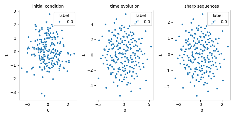
This figure shows our results with this numerical scheme. In the left=hand picture the initial condition, taken as a two-dimensional variate of a standard normal law. The figure in the middle displays the evolution at the time \(t=1\). The right-hand picture is a standard scaling of this last to unit variance.

Lagrangian()
plt.show()