Note
Go to the end to download the full example code.
9.04 GARCH(1,1) model
We reproduce here the figure 9.5 of the book. Utilitary functions can be found next to this file. Here, we only define codpy-related functions.
Necessary Imports
import os
import sys

import matplotlib.pyplot as plt
import numpy as np

from codpy.kernel import Sampler

try:
    CURRENT_DIR = os.path.dirname(os.path.abspath(__file__))
except NameError:
    CURRENT_DIR = os.getcwd()
data_path = os.path.join(CURRENT_DIR, "data")
PARENT_DIR = os.path.abspath(os.path.join(CURRENT_DIR, ".."))
sys.path.insert(0, PARENT_DIR)

import utils.ch9.mapping as maps
from utils.ch9.data_utils import stats_df
from utils.ch9.market_data import retrieve_market_data
from utils.ch9.path_generation import generate_paths
from utils.ch9.plot_utils import display_historical_vs_generated_distribution
Parameter definition
def get_cdpres_param():
    return {
        "rescale_kernel": {"max": 2000, "seed": None},
        "rescale": True,
        "grid_projection": True,
        "reproductibility": False,
        "date_format": "%d/%m/%Y",
        "begin_date": "01/06/2020",
        "end_date": "01/06/2022",
        "today_date": "01/06/2022",
        "symbols": ["AAPL", "GOOGL", "AMZN"],
    }
Get the market data
params = retrieve_market_data()
Defining the map
The GARCH(p,q) map is defined as:
\[\begin{split}\begin{aligned}
X^k &= \mu + \sigma^k \epsilon^k, \\
(\sigma^k)^2 &= \alpha_0 + \sum_{i=1}^{p} \alpha_i (X^{k-i})^2 + \sum_{j=1}^{q} \beta_j (\sigma^{k-j})^2,
\end{aligned}\end{split}\]
where \(\mu \in \mathbb{R}\), \(\{\epsilon^k\}\) is a white noise sequence with unit variance, and \(\sigma^k\) is a stochastic volatility term determined recursively.
The parameters \(\alpha_i\) and \(\beta_i\) denote the GARCH parameters.
q = 1


def garch_pq(x):
    import numpy as np
    from arch import arch_model

    p_values = range(1, 6)
    q_values = range(1, 6)
    aic_values = np.full((len(p_values), len(q_values)), np.inf)

    for i in p_values:
        for j in q_values:
            try:
                model = arch_model(x, vol="Garch", p=i, q=j)
                results = model.fit(disp="off")  # suppress convergence messages
                aic_values[i - 1, j - 1] = results.aic
            except:
                continue

    p, q = np.unravel_index(np.argmin(aic_values, axis=None), aic_values.shape)
    print(f"The smallest AIC is {aic_values[p, q]} for model GARCH({p}, {q})")

    best_p, best_q = p + 1, q + 1
    model = arch_model(x, vol="Garch", p=1, q=1)
    results = model.fit()
    print(results.summary())
    a0 = results.params["omega"]
    a = [
        results.params[f"alpha[{i+1}]"]
        for i in range(best_p)
        if f"alpha[{i+1}]" in results.params
    ]
    b = [
        results.params[f"beta[{i+1}]"]
        for i in range(best_q)
        if f"beta[{i+1}]" in results.params
    ]
    return a, b


def estimate_coeff():
    asx, bsx = [], []
    for i in range(params["data"].values.shape[1]):
        ax, bx = garch_pq(params["data"].values[:, i])
        asx += [ax]
        bsx += [bx]
    return np.asarray(asx).T, np.asarray(bsx).T


params["a"], params["b"] = estimate_coeff()
params["q"] = q
params["map"] = maps.composition_map(
    [maps.garch_map(), maps.mean_map(), maps.diff(), maps.log_map, maps.remove_time()]
)
params = maps.apply_map(params)
The smallest AIC is 4141.037702885732 for model GARCH(0, 0)
Iteration:      1,   Func. Count:      6,   Neg. LLF: 16986.629356658286
Iteration:      2,   Func. Count:     12,   Neg. LLF: 2988.1019261412503
Iteration:      3,   Func. Count:     18,   Neg. LLF: 2693.0760787188756
Iteration:      4,   Func. Count:     24,   Neg. LLF: 2100.2759470630394
Iteration:      5,   Func. Count:     30,   Neg. LLF: 2092.166149373335
Iteration:      6,   Func. Count:     36,   Neg. LLF: 2102.752613213072
Iteration:      7,   Func. Count:     42,   Neg. LLF: 2073.109754758848
Iteration:      8,   Func. Count:     47,   Neg. LLF: 2079.0329137844983
Iteration:      9,   Func. Count:     53,   Neg. LLF: 2069.501709914081
Iteration:     10,   Func. Count:     58,   Neg. LLF: 2068.2699961477
Iteration:     11,   Func. Count:     63,   Neg. LLF: 2067.5250950620048
Iteration:     12,   Func. Count:     68,   Neg. LLF: 2066.6828346716716
Iteration:     13,   Func. Count:     73,   Neg. LLF: 2066.542076310764
Iteration:     14,   Func. Count:     78,   Neg. LLF: 2066.5196720137887
Iteration:     15,   Func. Count:     83,   Neg. LLF: 2066.5189598207403
Iteration:     16,   Func. Count:     88,   Neg. LLF: 2066.518854345993
Iteration:     17,   Func. Count:     93,   Neg. LLF: 2066.518851442866
Iteration:     18,   Func. Count:     97,   Neg. LLF: 2066.5188514428664
Optimization terminated successfully    (Exit mode 0)
            Current function value: 2066.518851442866
            Iterations: 18
            Function evaluations: 97
            Gradient evaluations: 18
                     Constant Mean - GARCH Model Results
==============================================================================
Dep. Variable:                      y   R-squared:                       0.000
Mean Model:             Constant Mean   Adj. R-squared:                  0.000
Vol Model:                      GARCH   Log-Likelihood:               -2066.52
Distribution:                  Normal   AIC:                           4141.04
Method:            Maximum Likelihood   BIC:                           4157.94
                                        No. Observations:                  506
Date:              ven., août 22 2025   Df Residuals:                      505
Time:                        18:42:56   Df Model:                            1
                                 Mean Model
============================================================================
                 coef    std err          t      P>|t|      95.0% Conf. Int.
----------------------------------------------------------------------------
mu           125.5477      1.289     97.382      0.000 [1.230e+02,1.281e+02]
                              Volatility Model
===========================================================================
                 coef    std err          t      P>|t|     95.0% Conf. Int.
---------------------------------------------------------------------------
omega          3.7144      1.210      3.069  2.149e-03    [  1.342,  6.087]
alpha[1]       0.9041  9.503e-02      9.514  1.828e-21    [  0.718,  1.090]
beta[1]        0.0950  9.628e-02      0.987      0.324 [-9.370e-02,  0.284]
===========================================================================

Covariance estimator: robust
The smallest AIC is 3535.7251594871695 for model GARCH(0, 0)
Iteration:      1,   Func. Count:      6,   Neg. LLF: 602675894.7026879
Iteration:      2,   Func. Count:     12,   Neg. LLF: 2466.504882261799
Iteration:      3,   Func. Count:     19,   Neg. LLF: 1923.80528227795
Iteration:      4,   Func. Count:     25,   Neg. LLF: 1777.3978356491607
Iteration:      5,   Func. Count:     30,   Neg. LLF: 1770.7938839231458
Iteration:      6,   Func. Count:     35,   Neg. LLF: 1771.654547784799
Iteration:      7,   Func. Count:     41,   Neg. LLF: 1765.428021139962
Iteration:      8,   Func. Count:     46,   Neg. LLF: 1764.8287218853977
Iteration:      9,   Func. Count:     51,   Neg. LLF: 1764.4434332793412
Iteration:     10,   Func. Count:     56,   Neg. LLF: 1764.1555080824837
Iteration:     11,   Func. Count:     61,   Neg. LLF: 1763.8797244685038
Iteration:     12,   Func. Count:     66,   Neg. LLF: 1763.863264750603
Iteration:     13,   Func. Count:     71,   Neg. LLF: 1763.8625911283284
Iteration:     14,   Func. Count:     76,   Neg. LLF: 1763.8625797435848
Iteration:     15,   Func. Count:     80,   Neg. LLF: 1763.8625797422947
Optimization terminated successfully    (Exit mode 0)
            Current function value: 1763.8625797435848
            Iterations: 15
            Function evaluations: 80
            Gradient evaluations: 15
                     Constant Mean - GARCH Model Results
==============================================================================
Dep. Variable:                      y   R-squared:                       0.000
Mean Model:             Constant Mean   Adj. R-squared:                  0.000
Vol Model:                      GARCH   Log-Likelihood:               -1763.86
Distribution:                  Normal   AIC:                           3535.73
Method:            Maximum Likelihood   BIC:                           3552.63
                                        No. Observations:                  506
Date:              ven., août 22 2025   Df Residuals:                      505
Time:                        18:42:57   Df Model:                            1
                                 Mean Model
============================================================================
                 coef    std err          t      P>|t|      95.0% Conf. Int.
----------------------------------------------------------------------------
mu           161.9109      0.790    204.905      0.000 [1.604e+02,1.635e+02]
                               Volatility Model
=============================================================================
                 coef    std err          t      P>|t|       95.0% Conf. Int.
-----------------------------------------------------------------------------
omega          6.3218      1.499      4.218  2.466e-05      [  3.384,  9.259]
alpha[1]       0.9650  5.197e-02     18.568  5.800e-77      [  0.863,  1.067]
beta[1]        0.0350  3.141e-02      1.115      0.265 [-2.654e-02,9.660e-02]
=============================================================================

Covariance estimator: robust
The smallest AIC is 4340.552035447352 for model GARCH(0, 0)
Iteration:      1,   Func. Count:      6,   Neg. LLF: 16275.618037269702
Iteration:      2,   Func. Count:     13,   Neg. LLF: 2488.4649454939345
Iteration:      3,   Func. Count:     19,   Neg. LLF: 2213.4460017426973
Iteration:      4,   Func. Count:     25,   Neg. LLF: 2263.835511756241
Iteration:      5,   Func. Count:     31,   Neg. LLF: 2168.8691710334742
Iteration:      6,   Func. Count:     36,   Neg. LLF: 3108.6099731613394
Iteration:      7,   Func. Count:     42,   Neg. LLF: 2553.7899311915207
Iteration:      8,   Func. Count:     48,   Neg. LLF: 21964.18573516304
Iteration:      9,   Func. Count:     54,   Neg. LLF: 2168.38146506957
Iteration:     10,   Func. Count:     60,   Neg. LLF: 2166.5913578081636
Iteration:     11,   Func. Count:     65,   Neg. LLF: 2166.411205000175
Iteration:     12,   Func. Count:     70,   Neg. LLF: 2166.381080251631
Iteration:     13,   Func. Count:     75,   Neg. LLF: 2166.3639915405465
Iteration:     14,   Func. Count:     80,   Neg. LLF: 2166.3019670466983
Iteration:     15,   Func. Count:     85,   Neg. LLF: 2166.276311352476
Iteration:     16,   Func. Count:     90,   Neg. LLF: 2166.2760295185026
Iteration:     17,   Func. Count:     95,   Neg. LLF: 2166.276017723676
Iteration:     18,   Func. Count:     99,   Neg. LLF: 2166.2760178119124
Optimization terminated successfully    (Exit mode 0)
            Current function value: 2166.276017723676
            Iterations: 18
            Function evaluations: 99
            Gradient evaluations: 18
                     Constant Mean - GARCH Model Results
==============================================================================
Dep. Variable:                      y   R-squared:                       0.000
Mean Model:             Constant Mean   Adj. R-squared:                  0.000
Vol Model:                      GARCH   Log-Likelihood:               -2166.28
Distribution:                  Normal   AIC:                           4340.55
Method:            Maximum Likelihood   BIC:                           4357.46
                                        No. Observations:                  506
Date:              ven., août 22 2025   Df Residuals:                      505
Time:                        18:42:57   Df Model:                            1
                                 Mean Model
============================================================================
                 coef    std err          t      P>|t|      95.0% Conf. Int.
----------------------------------------------------------------------------
mu           114.6062      0.480    238.672      0.000 [1.137e+02,1.155e+02]
                            Volatility Model
========================================================================
                 coef    std err          t      P>|t|  95.0% Conf. Int.
------------------------------------------------------------------------
omega          2.7980      0.926      3.023  2.502e-03 [  0.984,  4.612]
alpha[1]       0.9983      0.149      6.709  1.964e-11 [  0.707,  1.290]
beta[1]    6.5511e-17      0.134  4.879e-16      1.000 [ -0.263,  0.263]
========================================================================

Covariance estimator: robust
We define our sampler on the mapped data using codpy’s Sampler
You can define your own latent generator function, here we use a simple uniform distribution. But if not provided, a default one will be used by the Sampler class.
mapped_data = params["transform_h"].values
generator = lambda n: np.random.uniform(size=(n, mapped_data.shape[1]))
sampler = Sampler(mapped_data, latent_generator=generator)
params["sampler"] = sampler
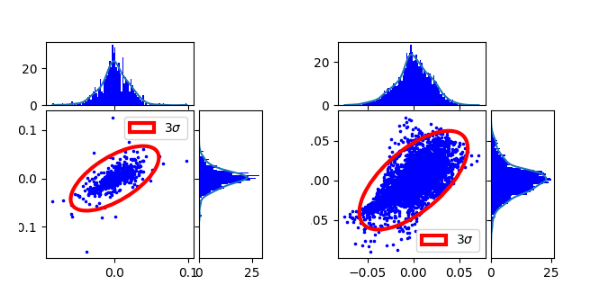
We plot the original distribution vs the generated one
params = display_historical_vs_generated_distribution(params)
params["graphic"](params)
plt.show()
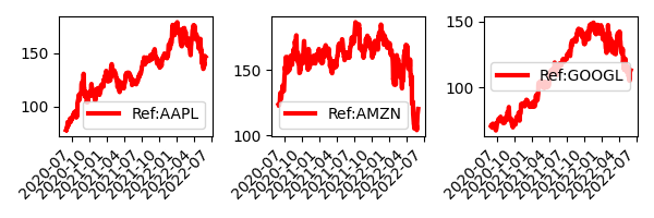
Reproductibility test
We regenerate the same path by generating from the latent representation We make sure we get the original data back.
params["reproductibility"] = True
params = generate_paths(params)
params["graphic"](params)
plt.show()
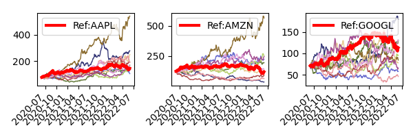
We now generate a new set of 10 paths
params["reproductibility"] = False
params["Nz"] = 10
params = generate_paths(params)
params["graphic"](params)
plt.show()

stats = stats_df(params["transform_h"], params["transform_g"]).T
print(stats)
                          0                  1                  2
Mean      -6.7e-06(0.00016)  -1.2e-06(2.7e-05)  -8.4e-06(0.00041)
Variance      -0.068(-0.24)       -0.44(0.076)      -0.089(-0.28)
Skewness    0.0004(0.00039)    0.0005(0.00043)   0.00033(0.00028)
Kurtosis            2(0.31)           6.7(1.1)           1.4(0.6)
KS test          0.54(0.05)         0.64(0.05)         0.72(0.05)
Total running time of the script: (0 minutes 4.835 seconds)