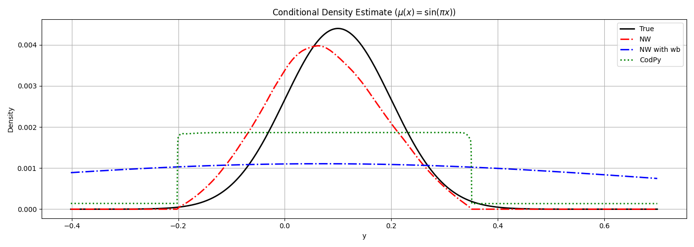
5.3.3 Kernel Conditional Density

We illustrate in this experiment the difference in density models of both the kernel-ridge and the Nadaraya-Watson approaches. To assess the ability to capture nonlinear patterns while estimating conditional densities, this experiment considers synthetic data from a heteroskedastic model, involving a uniform law \(X \sim \mathcal{U}(-1, 1)\), and a Gaussian one for \(Y\) with data

\[Y \mid X = x \sim \mathcal{N}(\mu(x), \sigma^2(x)), \quad \sigma(x) = 0.1 \cdot \cos\left(\frac{\pi x}{2}\right), \quad \mu(x) = \sin\left(\pi x\right).\]

Required imports

import matplotlib.pyplot as plt
import numpy as np
from scipy.stats import norm

import codpy.core
from codpy.conditioning import ConditionerKernel, NadarayaWatsonKernel
from codpy.core import kernel_setter
from codpy.utils import cartesian_outer_product, get_matrix

codpy.core.KerInterface.set_verbose()

Generating the data

The data is generated according to the chapter 5.3.3 of the book. - Illustrative example.

def mean_function_hard(x):
    return np.cos(np.pi / 2 * x)
    # return np.sin(np.pi * x)


def variance_function(x):
    return 0.1 * np.cos(np.pi * x * 0.5)


def mean_function(x):
    return 0.1 * np.cos(np.pi * x * 0.5)


def variance_function_hard(X):
    return 0.3 - 0.1 * mean_function(X)


def generate_conditional_hetero_skedastic_density_data(
    N_train=1000, seed=None, mean_f=None, variance_f=None
):
    """
    Generate synthetic data with nonlinear and heteroscedastic structure.

    Parameters:
    - N_train: Number of training samples (X, Y)
    - seed: Random seed for reproducibility
    - mean_f: Callable for mean function, e.g., mean_function(x)
    - variance_f: Callable for variance function, e.g., variance_function(x)

    Returns:
    - x: Training input samples (1D array)
    - y: Training output samples (1D array)
    - z: Test input sample (scalar)
    - y_pdf: Grid of y values for PDF estimation
    - (fz_mean, fz_std): True conditional mean and std at z
    - density: True conditional density at z over y_pdf
    """
    if seed is not None:
        np.random.seed(seed)

    if mean_f is None:
        mean_f = mean_function
    if variance_f is None:
        variance_f = variance_function

    x = np.random.uniform(-1.0, 1.0, N_train)
    mean_y = mean_f(x)
    std_y = variance_f(x)

    y = np.random.normal(loc=mean_y, scale=std_y)

    z = 0.0
    fz_mean = mean_f(z)
    fz_std = variance_f(z)

    y_pdf = np.linspace(2.0 * y.min(), 2.0 * y.max(), N_train)
    density = norm.pdf(y_pdf, loc=fz_mean, scale=fz_std)
    density /= density.sum(axis=0)

    return x, y, z, y_pdf, (fz_mean, fz_std), density


x, y, z, y_pdf, (fz_mean, fz_std), density = (
    generate_conditional_hetero_skedastic_density_data(
        N_train=1000,
        seed=None,
        mean_f=mean_function,
        variance_f=variance_function,
    )
)

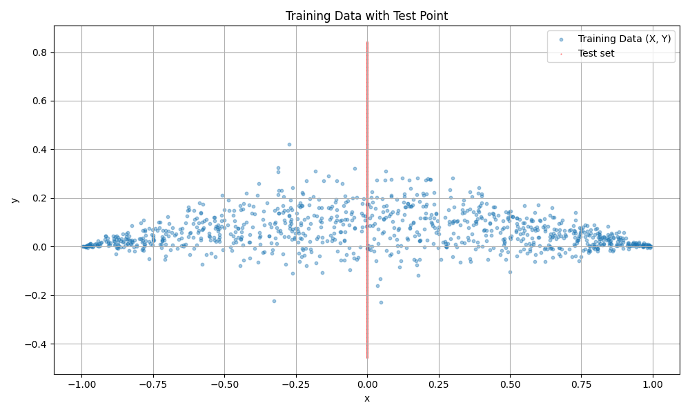
Plotting the data

We plot the data with the test points z and true conditional density p(y | z).

def plot_data_with_test_point(x, y, z, y_pdf):
    plt.figure(figsize=(10, 6))
    plt.scatter(x, y, alpha=0.4, label="Training Data (X, Y)", s=10)

    # Mark test point z
    out = cartesian_outer_product(get_matrix(z), get_matrix(y_pdf)).squeeze()
    plt.scatter(out[:, 0], out[:, 1], color="red", label="Test set", s=0.3, alpha=0.5)

    plt.title("Training Data with Test Point")
    plt.xlabel("x")
    plt.ylabel("y")
    plt.legend()
    plt.grid(True)
    plt.tight_layout()
    plt.show()


plot_data_with_test_point(x, y, z, y_pdf)

Estimators

We now use Nadaraya-Watson, CodPy’s Conditioner, and KDE to estimate the conditional density.

x, y, y_pdf, z = (
    x.reshape(-1, 1),
    y.reshape(-1, 1),
    y_pdf.reshape(-1, 1),
    np.array(z).reshape(-1, 1),
)


# For Kde, we use NadarayaWatsonKernel with the map set to bandwith.
nw = NadarayaWatsonKernel(
    x=x,
    y=y,
    set_kernel=kernel_setter(kernel_string="gaussian",kernel_args= {"bandwidth", 12}),
)
kde_result = nw.joint_density(y_pdf, z)
kde_result = kde_result.reshape(-1, 1)
kde_result /= kde_result.sum(axis=0)

# Without any specific kernel and maps, the default NadarayaWatson is used.

X_eval = np.linspace(-1, 1, 1000)
kde_bandwidth = 13
# kde_model = NadarayaWatsonKernel(
#     x=x, y=y, set_kernel=kernel_setter("gaussian", "bandwidth", bandwidth=kde_bandwidth)
# )
# mean_codpy = kde_model.expectation(
#     X_eval,
#     reg=0.1,
# )
codpy_model = ConditionerKernel(x=x, y=y)
mean_codpy = codpy_model.expectation(X_eval, reg=1.5)


# y_demeaned = y.reshape(-1, 1) - mean_codpy.reshape(-1, 1)

# nw = NadarayaWatsonKernel(x=x, y=y_demeaned)
nw = NadarayaWatsonKernel(x=x, y=y)
nw_result = nw.joint_density(y_pdf, z)
nw_result = nw_result.reshape(-1, 1)
nw_result /= nw_result.sum(axis=0)


codpy = ConditionerKernel(x=x, y=y)
codpy_result = codpy.get_transition(y=y_pdf, x=z)
codpy_result /= codpy_result.sum(axis=0)

Plotting the results

def plot_conditional_estimates(y_pdf, true_density, nw, kde, codpy, z):
    plt.figure(figsize=(10, 6))

    plt.plot(y_pdf, true_density, "k-", lw=2, label=f"True $p(y|z={z.item():.2f})$")
    plt.plot(y_pdf, nw, "r--", lw=2, label="Nadaraya-Watson")
    plt.plot(y_pdf, kde, "b-.", lw=2, label="Nadaraya-Watson (with bandwidth)")
    plt.plot(y_pdf, codpy, "g:", lw=2, label="CodPy ConditionerKernel")

    plt.title(f"Estimated Conditional Densities at z = {z.item():.2f}")
    plt.xlabel("y")
    plt.ylabel("Density")
    plt.legend()
    plt.grid(True)
    plt.tight_layout()


fig, axes = plt.subplots(1, 1, figsize=(14, 5))
X_eval = np.linspace(-1, 1, 1000)
kde_bandwidth = 13
z = np.array(0.0).reshape(-1, 1)


x, y, z_scalar, y_pdf, (fz_mean, fz_std), true_density = (
    generate_conditional_hetero_skedastic_density_data(
        N_train=1000,
        seed=3,
        mean_f=mean_function,
        variance_f=variance_function,
    )
)
y_pdf = y_pdf.reshape(-1, 1)
x = x.reshape(-1, 1)
y = y.reshape(-1, 1)
z = np.array(z_scalar).reshape(-1, 1)

# KDE with fixed bandwidth
kde_model = NadarayaWatsonKernel(
    x=x, y=y, set_kernel=kernel_setter(kernel_string="gaussian",kernel_args= {"bandwidth", 12})
)
kde_result = kde_model.joint_density(y_pdf, z)
kde_result /= kde_result.sum()

# Nadaraya-Watson with de-meaned residuals
nw_model = NadarayaWatsonKernel(x=x, y=y)
nw_result = nw_model.joint_density(y_pdf, z)
nw_result /= nw_result.sum()

# CodPy density estimate
codpy = ConditionerKernel(x=x, y=y)
codpy_result = codpy.get_transition(y=y_pdf, x=z)
codpy_result /= codpy_result.sum()

plt.plot(y_pdf, true_density, "k-", lw=2, label="True")
plt.plot(y_pdf, nw_result.reshape(-1, 1), "r-.", lw=2, label="NW")
plt.plot(y_pdf, kde_result.reshape(-1, 1), "b-.", lw=2, label="NW with wb")
plt.plot(y_pdf, codpy_result.reshape(-1, 1), "g:", lw=2, label="CodPy")

plt.title(r"Conditional Density Estimate ($\mu(x) = \sin(\pi x)$)")
plt.xlabel("y")
plt.ylabel("Density")
plt.grid(True)
plt.legend()

plt.tight_layout()
plt.show()

pass