3.4.4 Integral operator - inverse gradient operator

Given a kernel gradient operator ∇ₖ, CodPy defines an integral-type inverse operator denoted by:

\[ \nabla_k^{-1} = \Delta_k^{-1} \nabla_k^T \in \mathbb{R}^{N_x \times D N_z} \]

Matrix Interpretation

To compute this operator, the gradient tensor

\[ \nabla_k(\cdot, X) \in \mathbb{R}^{D \times N_z \times N_x} \]

is reshaped into a matrix of shape \(\mathbb{R}^{D N_z \times N_x}\).

Then, its transpose is multiplied by the inverse Laplacian \(\Delta_k^{-1}\) to obtain \(\nabla_k^{-1}\).

This operator acts on a vector field \(v_z \in \mathbb{R}^{D \times N_z \times D_{v_z}}\) and returns:

\[ \nabla_k^{-1}(\cdot, X) \cdot v_z \in \mathbb{R}^{N_x \times D_{v_z}}. \]

** Least-Squares Formulation **

Conceptually, this operation solves the following minimization problem:

\[ \bar{h} = \arg \min_{h \in \mathbb{R}^{N_x \times D_{v_z}}} \| \nabla_k h - v_z \|_{\ell^2}^2 \]

That is, it finds the best function \(h\) whose kernel gradient approximates a given vector field \(v_z\).

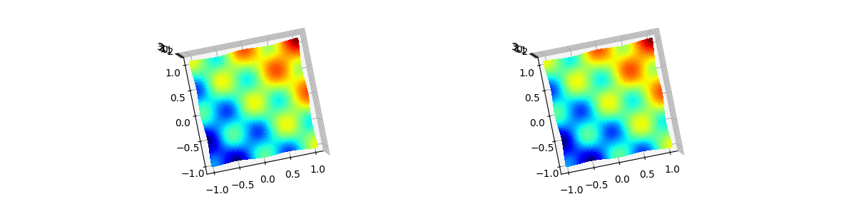
Example: 2D Case

In 2D, we can verify the behavior of the inverse by checking whether the composition:

\[ \nabla_k^{-1}(\cdot, X) \cdot \nabla_k(\cdot, X) f(X) \]

recovers the original function \(f(X)\).

This test confirms whether \(\nabla_k^{-1} \nabla_k\) approximates the identity.

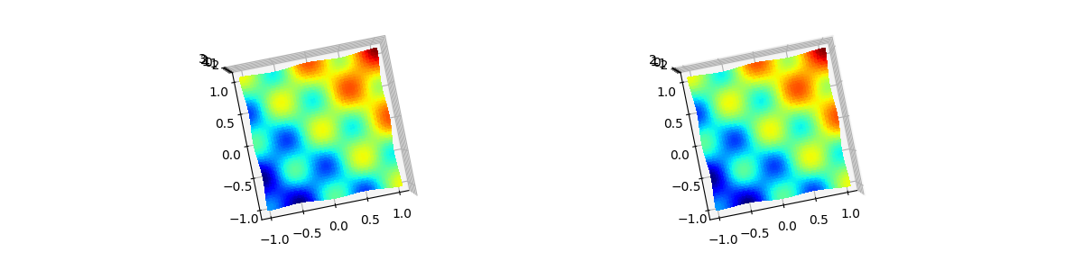
Extrapolation

We can also evaluate generalization by applying:

\[ \nabla_k^{-1}(\cdot, Z) \cdot \nabla_k(\cdot, X) f(X) \]

This measures how well the inverse-gradient operator extrapolates from \(X\) to unseen points \(Z\).

# Importing necessary modules
import os
import sys

from matplotlib import pyplot as plt

curr_f = os.path.join(os.getcwd(), "codpy-book", "utils")
sys.path.insert(0, curr_f)


import numpy as np

# from codpy.plotting import plot1D
# Lets import multi_plot function from codpy utils
from codpy.plot_utils import multi_plot


# Define the sinusoidal function
def periodic_fun(x):
    """
    A sinusoidal function that generates a sum of sines based on the input ``x``.
    """
    from math import pi

    sinss = np.cos(2 * x * pi)
    if x.ndim == 1:
        sinss = np.prod(sinss, axis=0)
        ress = np.sum(x, axis=0)
    else:
        sinss = np.prod(sinss, axis=1)
        ress = np.sum(x, axis=1)
    return ress + sinss


def nabla_my_fun(x):
    from math import pi

    import numpy as np

    sinss = np.cos(2 * x * pi)
    if x.ndim == 1:
        sinss = np.prod(sinss, axis=0)
        D = len(x)
        out = np.ones((D))

        def helper(d):
            out[d] += 2.0 * sinss * pi * np.sin(2 * x[d] * pi) / np.cos(2 * x[d] * pi)

        [helper(d) for d in range(0, D)]
    else:
        sinss = np.prod(sinss, axis=1)
        N = x.shape[0]
        D = x.shape[1]
        out = np.ones((N, D))

        def helper(d):
            out[:, d] += (
                2.0 * sinss * pi * np.sin(2 * x[:, d] * pi) / np.cos(2 * x[:, d] * pi)
            )

        [helper(d) for d in range(0, D)]
    return out


# Function to generate periodic data
def generate_periodic_data_cartesian(size_x, size_z, fun=None, nabla_fun=None):
    """
    Generates 2D structured Cartesian grid data for x and z domains,
    and evaluates a given function and optionally its gradient.

    Parameters:
    - size_x: number of points per axis for x (grid will be size_x^2)
    - size_z: number of points per axis for z (grid will be size_z^2)
    - fun: function to evaluate at each point
    - nabla_fun: optional gradient function to evaluate

    Returns:
    - x, z: 2D Cartesian grids of shape (N, 2)
    - fx, fz: function values at x and z
    - nabla_fx, nabla_fz (if nabla_fun is provided)
    """

    def cartesian_grid(size, box):
        lin = [np.linspace(box[0, d], box[1, d], size) for d in range(2)]
        X, Y = np.meshgrid(*lin)
        return np.stack([X.ravel(), Y.ravel()], axis=1)

    # Define domain boxes
    X_box = np.array([[-1, -1], [1, 1]])
    Z_box = np.array([[-1.5, -1.5], [1.5, 1.5]])

    # Generate Cartesian grids
    x = cartesian_grid(size_x, X_box)
    z = cartesian_grid(size_z, Z_box)

    # Function evaluations
    fx = fun(x).reshape(-1, 1) if fun else None
    fz = fun(z).reshape(-1, 1) if fun else None

    if nabla_fun:
        nabla_fx = nabla_fun(x)
        nabla_fz = nabla_fun(z)
        return x, fx, z, fz, nabla_fx, nabla_fz

    return x, fx, z, fz


# Lets define helper function to plot 3D projection of the function
def plot_trisurf(xfx, ax, legend="", elev=90, azim=-100, **kwargs):
    from matplotlib import cm

    """
    Helper function to plot a 3D surface using a trisurf plot.

    Parameters:
    - xfx: A tuple containing the x-coordinates (2D points) and their
      corresponding function values.
    - ax: The matplotlib axis object for plotting.
    - legend: The legend/title for the plot.
    - elev, azim: Elevation and azimuth angles for the 3D view.
    - kwargs: Additional keyword arguments for further customization.
    """

    xp, fxp = xfx[0], xfx[1]
    x, fx = xp, fxp

    X, Y = x[:, 0], x[:, 1]
    Z = fx.flatten()
    ax.plot_trisurf(X, Y, Z, antialiased=False, cmap=cm.jet)
    ax.view_init(azim=azim, elev=elev)
    ax.title.set_text(legend)


# import CodPy's core module and Kernel class
from codpy import core
from codpy.kernel import Kernel

Integral operator - inverse gradient operator

---

def fun_NablainvNabla1(size_x=50, size_y=50):
    x, fx, z, fz, _, nabla_fz = generate_periodic_data_cartesian(
        size_x, size_y, periodic_fun, nabla_fun=nabla_my_fun
    )

    nabla_fz = nabla_fz.reshape(-1, 2, 1)

    kernel_ptr = Kernel(
        x=x, fx=fx, set_kernel=core.kernel_setter("tensornorm", "scale_to_unitcube")
    ).get_kernel()

    fz_inv = core.DiffOps.nabla_inv(
        x=x,
        y=x,
        z=x,
        kernel_ptr=kernel_ptr,
        fz=core.DiffOps.nabla(x=x, y=x, z=x, fx=fx, kernel_ptr=kernel_ptr),
    )
    multi_plot(
        [(x, fx), (x, fz_inv)],
        plot_trisurf,
        projection="3d",
        mp_nrows=1,
        mp_figsize=(12, 3),
        mp_titles=[
            "Comparison between original function to the product of the gradient operator and its inverse"
        ],
    )
    plt.show()


fun_NablainvNabla1()


def fun_NablainvNabla2(size_x=50, size_y=50):
    x, fx, z, fz, _, nabla_fz = generate_periodic_data_cartesian(
        size_x, size_y, periodic_fun, nabla_fun=nabla_my_fun
    )

    nabla_fz = nabla_fz.reshape(-1, 2, 1)

    kernel_ptr = Kernel(
        x=x, fx=fx, set_kernel=core.kernel_setter("tensornorm", "scale_to_unitcube")
    ).get_kernel()

    fz_inv = core.DiffOps.nabla_inv(
        x=x,
        y=x,
        z=z,
        kernel_ptr=kernel_ptr,
        fz=core.DiffOps.nabla(x=x, y=x, z=z, fx=fx, kernel_ptr=kernel_ptr),
    )
    multi_plot(
        [(x, fx), (x, fz_inv)],
        plot_trisurf,
        projection="3d",
        mp_nrows=1,
        mp_figsize=(12, 3),
        mp_titles=[
            "Comparison between original function to the product of the inverse of the gradient operator and the gradient operator"
        ],
    )
    plt.show()


fun_NablainvNabla2()

• 
•