5.6.b Application of OT in Disitribution Sampling : 2D

We repeat the previous test in one dimension with two-dimensional data, and present scatter plots of the original and generated data for each of the two cases, allowing a visual comparison of the fidelity of the generative process.

import numpy as np
import pandas as pd
from matplotlib import pyplot as plt

from codpy import core
from codpy.kernel import Kernel, Sampler


def normal_wrapper(center, size, radius=1.0, **kwargs):
    return np.random.normal(loc=center, scale=radius, size=size)


def student_wrapper(center, size, **kwargs):
    df = kwargs.get("df", 3.0)
    out = np.random.standard_t(df, size=size)
    out += center
    return out


def generate_multimodal_data(
    N=500,
    D=1,
    num_clusters=2,
    centers=None,
    radii=None,
    weights=None,
    random_variable=None,
    **kwargs,
):
    """
    Generate synthetic multimodal data from a mixture of clusters.

    Parameters:
        N (int): Total number of samples.
        D (int): Dimensionality of the data.
        num_clusters (int): Number of clusters.
        centers (np.ndarray): Optional. Shape (num_clusters, D).
        radii (np.ndarray): Optional. Std dev per cluster.
        weights (np.ndarray): Optional. Cluster weights (should sum to 1).
        random_variable (callable): Custom sampling function. Default is np.random.normal.

    Returns:
        x (pd.DataFrame): Data samples.
        labels (pd.Series): Cluster labels for each sample.
    """
    if centers is None:
        centers = np.random.normal(loc=0.0, scale=0.5, size=(num_clusters, D))
        centers -= centers.mean(axis=0)
        centers = centers * 4./np.linalg.norm(centers, axis=1, keepdims=True)

    if radii is None:
        radii = np.abs(np.random.normal(loc=0.2, scale=0.1, size=num_clusters))

    if weights is None:
        weights = np.ones(num_clusters) / num_clusters

    if random_variable is None:
        random_variable = normal_wrapper

    x_list, label_list = [], []

    for i in range(num_clusters):
        num_samples = int(N * weights[i])
        samples = random_variable(
            center=centers[i], size=(num_samples, D), radius=radii[i], **kwargs
        )
        x_list.append(samples)
        label_list.extend([i] * num_samples)

    x = pd.DataFrame(np.vstack(x_list), columns=[f"dim_{d}" for d in range(D)])
    labels = pd.Series(label_list, name="cluster")
    return x, labels


def df_summary(df):
    return pd.DataFrame(
        {
            "Mean": df.mean(),
            "Variance": df.var(),
            "Skewness": df.skew(),
            "Kurtosis": df.kurtosis(),
        }
    )


from scipy.stats import ks_2samp


def ks_testD(x, y, alpha=0.05):
    """
    Performs Kolmogorov-Smirnov test for each dimension.

    Parameters:
        x (np.ndarray or pd.DataFrame): First sample.
        y (np.ndarray or pd.DataFrame): Second sample.
        alpha (float): Significance level (default 0.05).

    Returns:
        pd.Series: p-values from the KS test.
        pd.Series: Constant threshold values (same for all dimensions).
    """
    x = x.values if isinstance(x, pd.DataFrame) else x
    y = y.values if isinstance(y, pd.DataFrame) else y

    D = x.shape[1]
    p_values = []
    thresholds = []

    for i in range(D):
        stat = ks_2samp(x[:, i], y[:, i])
        p_values.append(stat.pvalue)
        thresholds.append(alpha)  # Optional: could vary if computed per dim

    return pd.Series(p_values, name="p-value"), pd.Series(thresholds, name="threshold")


def stats_df(dfx_list, dfy_list, f_names=None, fmt="{:.2g}"):
    """
    Computes and formats summary statistics between reference and sampled data.

    Parameters:
        dfx_list (list): List of reference datasets (np.ndarray or pd.DataFrame).
        dfy_list (list): List of sampled datasets (np.ndarray or pd.DataFrame).
        f_names (list): Optional. Row labels. Should match total number of columns across all datasets.
        fmt (str): Format string for floats.

    Returns:
        pd.DataFrame: Formatted summary statistics.
    """

    if not isinstance(dfx_list, list):
        dfx_list = [dfx_list]
    if not isinstance(dfy_list, list):
        dfy_list = [dfy_list]

    def format_pair(x_vals, y_vals):
        return [f"{fmt.format(x)} ({fmt.format(y)})" for x, y in zip(x_vals, y_vals)]

    all_stats, full_index = [], []
    for i, (dfx, dfy) in enumerate(zip(dfx_list, dfy_list)):
        dfx = pd.DataFrame(dfx)
        dfy = pd.DataFrame(dfy)

        sx, sy = df_summary(dfx), df_summary(dfy)
        ks_df, ks_thr = ks_testD(dfx, dfy)

        stats = {
            "Mean": format_pair(sx.Mean, sy.Mean),
            "Variance": format_pair(sx.Variance, sy.Variance),
            "Skewness": format_pair(sx.Skewness, sy.Skewness),
            "Kurtosis": format_pair(sx.Kurtosis, sy.Kurtosis),
            "KS test": format_pair(ks_df, ks_thr),
        }

        all_stats.append(pd.DataFrame(stats, index=dfx.columns))
        if f_names and i < len(f_names):
            full_index.extend([f"{f_names[i]}:{col}" for col in dfx.columns])
        else:
            full_index.extend(dfx.columns)

    result = pd.concat(all_stats)
    result.index = full_index
    return result

Two-dimensional illustrations

---

def compare_distributions_2d(N=300, Nz=500):
    """
    Compare Gaussian and Student-t distributions using 2D sampling and scatter plotting.
    """

    def scatter_plot(ref, sampled, ax=None, title=""):
        if ax is None:
            ax = plt.gca()
        ax.scatter(ref[:, 0], ref[:, 1], alpha=0.4, label="Reference")
        ax.scatter(sampled[:, 0], sampled[:, 1], alpha=0.4, label="Sampled")
        ax.set_title(title)
        ax.legend()

    # Generate Gaussian data
    y_gauss_df, _ = generate_multimodal_data(N=N, D=2)
    y_gauss = y_gauss_df.values
    sampler_gauss = Sampler(y_gauss,reg=0.,distance=None)
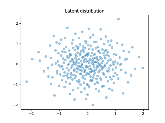
    plt.scatter(sampler_gauss.x[:, 0], sampler_gauss.x[:, 1], alpha=0.4, label="Reference Gaussian")
    plt.title("Latent distribution")
    plt.show()
    sampled_gauss = sampler_gauss.sample(Nz)
    # sampled_gauss = sampler_gauss.get_fx()

    # Generate Student-t data
    y_student_df, _ = generate_multimodal_data(
        N=N, D=2, random_variable=student_wrapper
    )
    y_student = y_student_df.values
    sampler_student = Sampler(y_student)
    sampled_student = sampler_student.sample(Nz)

    # Plot
    fig, axes = plt.subplots(1, 2, figsize=(12, 5))
    scatter_plot(y_gauss, sampled_gauss, ax=axes[0], title="Gaussian Distribution")
    scatter_plot(y_student, sampled_student, ax=axes[1], title="Student-t Distribution")
    plt.tight_layout()
    plt.show()

    return stats_df(
        [y_gauss, y_student],
        [sampled_gauss, sampled_student],
        f_names=["Gaussian", "Student-t"],
    )
core.KerInterface.set_verbose()

stats = compare_distributions_2d()
stats.to_latex(
    "ch5_6_b.tex",
    index=True,
    float_format="%.2g",
    caption="Comparison of Gaussian and Student-t distributions using 1D sampling.",
    label="tab:ch5_6_b",
)
print(stats)
pass

• 
• 

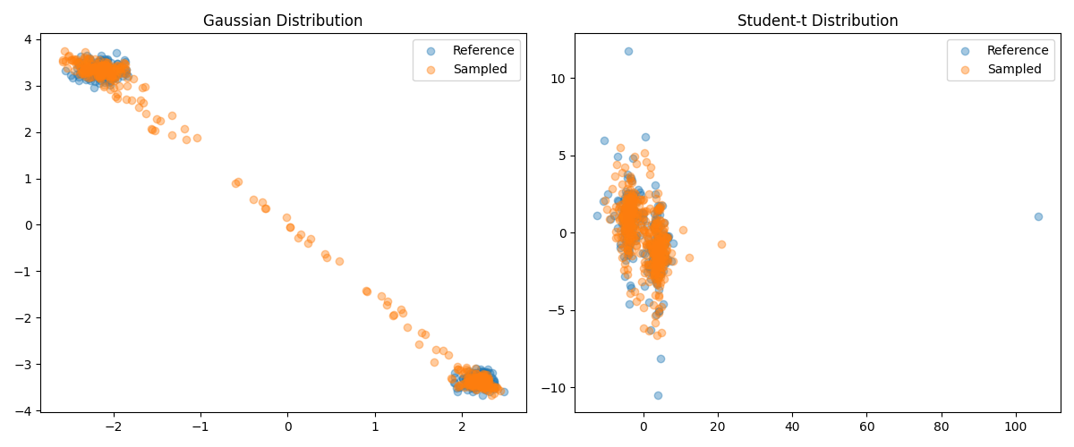
                        Mean   Variance          Skewness         Kurtosis      KS test
Gaussian:0   0.01 (-0.00037)  4.7 (4.4)  -0.0029 (0.0078)        -2 (-1.9)  0.58 (0.05)
Gaussian:1    -0.015 (0.004)    11 (11)    0.001 (-0.012)        -2 (-1.9)   0.4 (0.05)
Student-t:0      0.3 (0.058)    55 (18)        9.7 (0.17)  1.4e+02 (-0.17)  0.99 (0.05)
Student-t:1    -0.13 (-0.16)  4.5 (3.5)     0.021 (-0.26)       5.3 (0.66)     1 (0.05)