Note
Go to the end to download the full example code.
2.3 1D Periodic Function Extrapolation
In this experiment, we explore various machine learning and interpolation techniques to model and predict a sinusoidal function. We use different models, including CodPy, SciPy’s RBF interpolator, Scikit-learn’s SVR, Decision Trees, AdaBoost, Random Forest, Feedforward Neural Network, and XGBoost.
Objective
The goal of this experiment is to compare the performance of different models
in predicting the output of a complex sinusoidal function (periodic_fun). The function
is defined over a range of input values (x), and we generate predictions over
a broader range (z) to see how each model generalizes beyond the training data.
Data Generation
We define a sinusoidal function periodic_fun and use it to generate the target values (fx)
for a set of input values x ranging from -1 to 1. We generate a broader range of test inputs
(z) ranging from -1.5 to 1.5 for evaluating the models.
Steps:
Define a periodic sinusoidal function,
periodic_fun.Generate input data (
x) and evaluate the function to obtain target values (fx).Generate test data (
z) over a broader range to evaluate model predictions beyond the training data.Train different models using the input data (
x,fx) and predict values over the test range (z).Visualize the predictions from each model in a grid format for comparison.
# Importing necessary modules
import os
import sys
import time

curr_f = os.path.join(os.getcwd(), "codpy-book", "utils")
sys.path.insert(0, curr_f)


import matplotlib.pyplot as plt
import numpy as np

# from codpy.plotting import plot1D
# Lets import multi_plot function from codpy utils
from codpy.plot_utils import multi_plot, plot1D
from sklearn.metrics import mean_squared_error


# Define the sinusoidal function
def periodic_fun(x):
    """
    A sinusoidal function that generates a sum of sines based on the input ``x``.
    """
    from math import pi

    sinss = np.cos(2 * x * pi)
    if x.ndim == 1:
        sinss = np.prod(sinss, axis=0)
        ress = np.sum(x, axis=0)
    else:
        sinss = np.prod(sinss, axis=1)
        ress = np.sum(x, axis=1)
    return ress + sinss


def periodicdata1D():
    # lets define a simple 1D periodic data function
    x = np.linspace(-1, 1, 100).reshape(-1, 1)
    z = np.linspace(-1.5, 1.5, 100).reshape(-1, 1)
    fx = np.array([periodic_fun(np.array([i])) for i in x])
    fz = np.array([periodic_fun(np.array([i])) for i in z])
    # Plot the data for x and z
    multi_plot([(x, fx), (z, fz)], plot1D, mp_nrows=1, mp_figsize=(12, 3))


# Call the function to generate and plot the data
periodicdata1D()
plt.show()
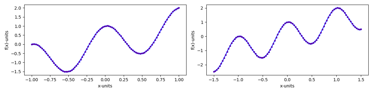
The plot shows a sinusoidal pattern for the data generated in the cartesian coordinate system.
The two curves for x and z exhibits the sinusoidal variations defined by periodic_fun(x).
Model Setup and Training
We use several models, each wrapped as a function for modularity:
CodPy Model: Uses the CodPy library’s kernel regression model with a specified kernel.
RBF Interpolator (SciPy): A radial basis function interpolator that uses a multiquadric kernel.
SVR (Scikit-learn): Support Vector Regressor using a radial basis function (RBF) kernel.
Neural Network (Pytorch): A simple feedforward neural network with two hidden layers.
Decision Tree (Scikit-learn): A decision tree regressor with a maximum depth of 10.
AdaBoost (Scikit-learn): An AdaBoost model with a decision tree as the base estimator.
XGBoost: A gradient-boosted tree model from the XGBoost library.
Random Forest (Scikit-learn): An ensemble of decision trees trained with random subsets of the data.
Prediction
Each model is trained on the generated dataset (
x,fx) and then used to predict the values over the test range (z). The predictions (fz) are stored and transformed into a compatible format for plotting.
Expected Output
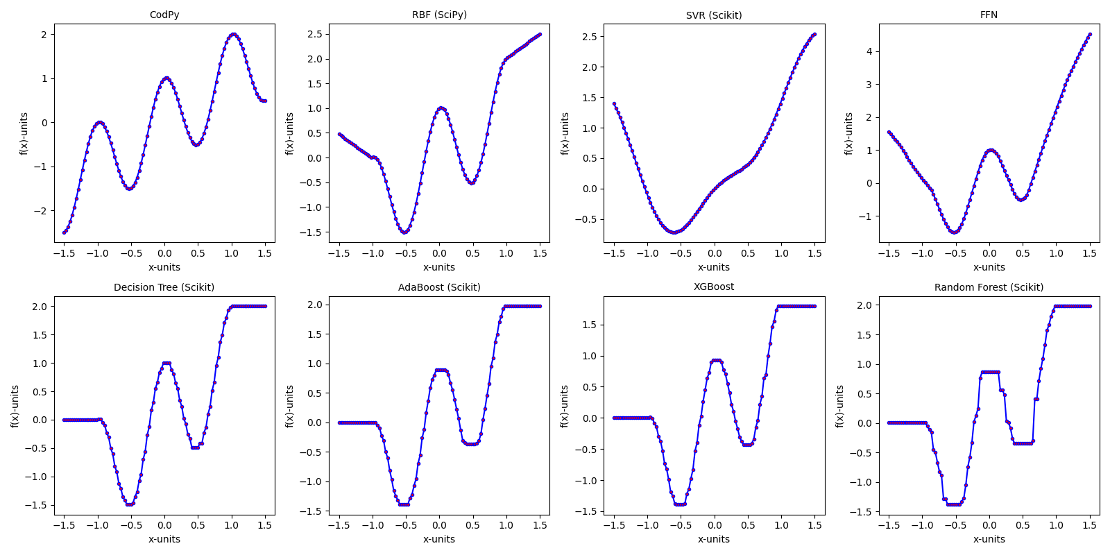
The output consists of a 2x4 grid of plots, where each plot displays the predictions from one of the models compared to the underlying function. The aim is to observe differences in accuracy and generalization ability between models, especially beyond the training range.
# First we import necessary libraries
# import CodPy's core module and Kernel class
from codpy import core
from codpy.kernel import Kernel
from scipy.interpolate import Rbf
from sklearn.ensemble import AdaBoostRegressor, RandomForestRegressor
from sklearn.svm import SVR
from sklearn.tree import DecisionTreeRegressor
from xgboost import XGBRegressor
# Model functions
# 0. CodPy
def codpy_model(x, fx, z):
kernel = Kernel(
set_kernel=core.kernel_setter("gaussianper", None,2,1e-9), x=x, fx=fx, order=2
)
res = kernel(z)
mmd = np.sqrt(kernel.discrepancy(z))
return res, mmd
# 1. SciPy RBF Interpolator
def rbf_interpolator(x, fx, z):
rbf = Rbf(x.ravel(), fx.ravel(), function="multiquadric")
return rbf(z.ravel()), None
# 2. Scikit-learn SVR
def svr_model(x, fx, z):
svr = SVR(kernel="rbf", gamma="auto", C=1)
svr.fit(x, fx.ravel())
return svr.predict(z), None
# 3. NN
import torch
import torch.nn as nn
import torch.optim as optim
from torch.utils.data import DataLoader, TensorDataset, random_split
class FFN(nn.Module):
def __init__(
self, in_features, hidden_features=64, hidden_layers=3, out_features=1
):
super().__init__()
layers = []
layers.append(nn.Linear(in_features, hidden_features))
layers.append(nn.ReLU())
for _ in range(hidden_layers - 1):
layers.append(nn.Linear(hidden_features, hidden_features))
layers.append(nn.ReLU())
layers.append(nn.Linear(hidden_features, out_features))
self.net = nn.Sequential(*layers)
def forward(self, x):
return self.net(x)
def neural_network(x, fx, z):
x_tensor = torch.tensor(x, dtype=torch.float32)
fx_tensor = torch.tensor(fx, dtype=torch.float32).view(-1, 1)
z_tensor = torch.tensor(z, dtype=torch.float32)
dataset = TensorDataset(x_tensor, fx_tensor)
val_size = int(0.1 * len(dataset))
train_size = len(dataset) - val_size
train_dataset, val_dataset = random_split(dataset, [train_size, val_size])
train_loader = DataLoader(train_dataset, batch_size=16, shuffle=True)
val_loader = DataLoader(val_dataset, batch_size=16)
model = FFN(in_features=1, hidden_features=64, hidden_layers=3, out_features=1)
# loss and optimizer
criterion = nn.MSELoss()
optimizer = optim.Adam(model.parameters(), lr=0.001)
model.train()
for epoch in range(150):
for batch_x, batch_y in train_loader:
optimizer.zero_grad()
outputs = model(batch_x)
loss = criterion(outputs, batch_y)
loss.backward()
optimizer.step()
model.eval()
with torch.no_grad():
predictions = model(z_tensor).flatten().numpy()
return predictions, None
# 4. Decision Tree Regressor
def decision_tree(x, fx, z):
tree = DecisionTreeRegressor(max_depth=10)
tree.fit(x, fx.ravel())
return tree.predict(z), None
# 5. AdaBoost Regressor
def adaboost_model(x, fx, z):
ada = AdaBoostRegressor(
DecisionTreeRegressor(max_depth=5), n_estimators=50, learning_rate=1
)
ada.fit(x, fx.ravel())
return ada.predict(z), None
# 6. XGBoost Regressor
def xgboost_model(x, fx, z):
xgb = XGBRegressor(max_depth=5, n_estimators=10)
xgb.fit(x, fx.ravel())
return xgb.predict(z), None
# 7. Random Forest Regressor
def random_forest(x, fx, z):
rf = RandomForestRegressor(max_depth=5, n_estimators=5)
rf.fit(x, fx.ravel())
return rf.predict(z), None
# List of model functions
model_functions = [
codpy_model,
rbf_interpolator,
svr_model,
neural_network,
decision_tree,
adaboost_model,
xgboost_model,
random_forest,
]
def plot_models():
"""
This function generates random data for x and z coordinates, applies each model
in `model_functions` to generate predictions, and plots the results using `multi_plot`.
"""
# Generate x and z data
x = np.linspace(-1, 1, 100).reshape(-1, 1)
z = np.linspace(-1.5, 1.5, 100).reshape(-1, 1)
# Apply the periodic function to generate fx and fz values
fx = np.array([periodic_fun(np.array([i])) for i in x])
fz = np.array([periodic_fun(np.array([i])) for i in z])
# Generate predictions for each model in the model_functions list
list_of_results = [model(x, fx, z) for model in model_functions]
# Titles for each subplot
title_list = [
"CodPy",
"RBF (SciPy)",
"SVR (Scikit)",
"FFN",
"Decision Tree (Scikit)",
"AdaBoost (Scikit)",
"XGBoost",
"Random Forest (Scikit)",
]
# Use a lambda function to transform z and fz into (z, fz) tuples
zfz_transform = lambda z, fz: (z.ravel(), fz.ravel())
# Apply the transformation to each model's output
transformed_results = [zfz_transform(z, result) for result, _ in list_of_results]
# Create the multi-plot visualization
multi_plot(
transformed_results,
plot1D,
f_names=title_list,
mp_max_items=8,
mp_nrows=2,
mp_ncols=4,
mp_figsize=(16, 8),
)
plt.show()
Nxs = np.arange(start=10, stop=len(x) + 1, step=(len(x) - 10) // 5)
results = {}
times = {}
mmds = {}
for Nx in Nxs:
results[Nx] = {}
times[Nx] = {}
mmds[Nx] = {}
for i, model in enumerate(model_functions):
start = time.perf_counter()
f_z, mmd = model(x[:Nx], fx[:Nx], z)
end = time.perf_counter()
mmds[Nx][title_list[i]] = mmd
results[Nx][title_list[i]] = mean_squared_error(fz, f_z)
times[Nx][title_list[i]] = end - start
print(f"Model: {title_list[i]}, Time taken: {end-start:.4f} seconds")
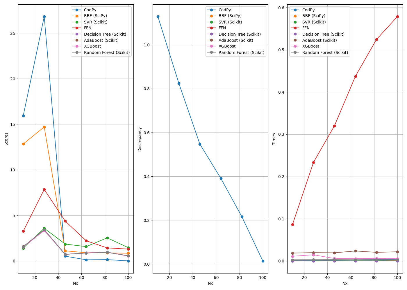
res = [{"data": results}, {"data": mmds}, {"data": times}]
def plot_one(inputs):
results = inputs["data"]
ax = inputs["ax"]
legend = inputs["legend"]
for model_name in next(iter(results.values())).keys():
x_vals = sorted(results.keys())
y_vals = [results[x][model_name] for x in x_vals]
ax.plot(x_vals, y_vals, marker="o", label=model_name)
ax.set_xlabel("Nx")
ax.set_ylabel(legend)
ax.legend()
ax.grid(True)
multi_plot(
res,
plot_one,
mp_nrows=1,
mp_ncols=3,
legends=["Scores", "Discrepancy", "Times"],
mp_figsize=(14, 10),
)
plt.show()
# Lets plot the models
plot_models()
Model: CodPy, Time taken: 0.0016 seconds
Model: RBF (SciPy), Time taken: 0.0002 seconds
Model: SVR (Scikit), Time taken: 0.0002 seconds
Model: FFN, Time taken: 0.0865 seconds
Model: Decision Tree (Scikit), Time taken: 0.0002 seconds
Model: AdaBoost (Scikit), Time taken: 0.0187 seconds
Model: XGBoost, Time taken: 0.0111 seconds
Model: Random Forest (Scikit), Time taken: 0.0029 seconds
Model: CodPy, Time taken: 0.0017 seconds
Model: RBF (SciPy), Time taken: 0.0002 seconds
Model: SVR (Scikit), Time taken: 0.0003 seconds
Model: FFN, Time taken: 0.2336 seconds
Model: Decision Tree (Scikit), Time taken: 0.0002 seconds
Model: AdaBoost (Scikit), Time taken: 0.0197 seconds
Model: XGBoost, Time taken: 0.0146 seconds
Model: Random Forest (Scikit), Time taken: 0.0030 seconds
Model: CodPy, Time taken: 0.0020 seconds
Model: RBF (SciPy), Time taken: 0.0003 seconds
Model: SVR (Scikit), Time taken: 0.0005 seconds
Model: FFN, Time taken: 0.3201 seconds
Model: Decision Tree (Scikit), Time taken: 0.0002 seconds
Model: AdaBoost (Scikit), Time taken: 0.0193 seconds
Model: XGBoost, Time taken: 0.0058 seconds
Model: Random Forest (Scikit), Time taken: 0.0032 seconds
Model: CodPy, Time taken: 0.0028 seconds
Model: RBF (SciPy), Time taken: 0.0003 seconds
Model: SVR (Scikit), Time taken: 0.0007 seconds
Model: FFN, Time taken: 0.4375 seconds
Model: Decision Tree (Scikit), Time taken: 0.0003 seconds
Model: AdaBoost (Scikit), Time taken: 0.0237 seconds
Model: XGBoost, Time taken: 0.0057 seconds
Model: Random Forest (Scikit), Time taken: 0.0030 seconds
Model: CodPy, Time taken: 0.0033 seconds
Model: RBF (SciPy), Time taken: 0.0004 seconds
Model: SVR (Scikit), Time taken: 0.0009 seconds
Model: FFN, Time taken: 0.5243 seconds
Model: Decision Tree (Scikit), Time taken: 0.0002 seconds
Model: AdaBoost (Scikit), Time taken: 0.0204 seconds
Model: XGBoost, Time taken: 0.0059 seconds
Model: Random Forest (Scikit), Time taken: 0.0031 seconds
Model: CodPy, Time taken: 0.0042 seconds
Model: RBF (SciPy), Time taken: 0.0006 seconds
Model: SVR (Scikit), Time taken: 0.0022 seconds
Model: FFN, Time taken: 0.5787 seconds
Model: Decision Tree (Scikit), Time taken: 0.0003 seconds
Model: AdaBoost (Scikit), Time taken: 0.0217 seconds
Model: XGBoost, Time taken: 0.0056 seconds
Model: Random Forest (Scikit), Time taken: 0.0030 seconds
Total running time of the script: (0 minutes 4.135 seconds)