7.05 Convex Hull Algorithm

We reproduce here the figure 7.7 & 7.8 of the book. Utilitary functions can be found next to this file. Here, we only define codpy-related functions.

Necessary Imports

import os
import sys

import matplotlib.pyplot as plt

try:
    CURRENT_DIR = os.path.dirname(os.path.abspath(__file__))
except NameError:
    CURRENT_DIR = os.getcwd()
data_path = os.path.join(CURRENT_DIR, "data")
PARENT_DIR = os.path.abspath(os.path.join(CURRENT_DIR, ".."))
sys.path.insert(0, PARENT_DIR)

from utils.ch7.ch7_utils import CHA1D, CHA2D

Problem statement

We consider the Convex Hull algorithm and compute

\[u(t,\cdot) = y^+(t,\cdot)_\# u_0(\cdot), \quad y(t,x) = x + t f'(u_0(x)),\]

Where \(y^+(t,\cdot)\) is computed as

\[y^+(t,\cdot) = \nabla h^+(t,\cdot), \quad \nabla h(t,\cdot) = y(t,\cdot),\]

and \(h^+(t,\cdot)\) is the convex hull of \(h\).

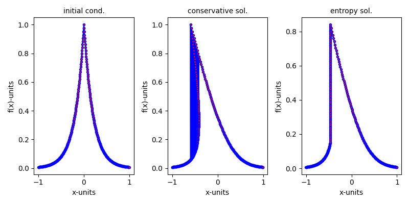
One dimensional

This figures illustrates this computation for the one-dimensional Burgers equation :

\[\partial_t u + \frac{1}{2}\partial_x u^2 =0,\]

The left-hand figure is the initial condition at time zero, since the solution at middle represent the conservative solution at time 1, and the entropy solution is plot at right.

CHA1D()
plt.show()

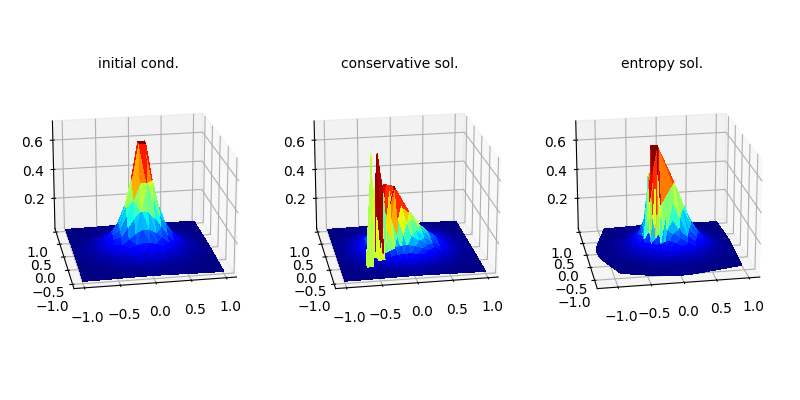
Two dimensional

This figures illustrates the two dimensional case :

\[\partial_t u + \frac{1}{2}\nabla \cdot(u^2,u^2)=0\]

CHA2D()
plt.show()
pass