9.08 Stochastic volatility model

We reproduce here the figure 9.9 of the book. Utilitary functions can be found next to this file. Here, we only define codpy-related functions.

Necessary Imports

import os
import sys

import matplotlib.pyplot as plt
import numpy as np

from codpy.kernel import Sampler

try:
    CURRENT_DIR = os.path.dirname(os.path.abspath(__file__))
except NameError:
    CURRENT_DIR = os.getcwd()
data_path = os.path.join(CURRENT_DIR, "data")
PARENT_DIR = os.path.abspath(os.path.join(CURRENT_DIR, ".."))
sys.path.insert(0, PARENT_DIR)

import utils.ch9.mapping as maps
from utils.ch9.market_data import retrieve_market_data
from utils.ch9.path_generation import generate_paths
from utils.ch9.plot_utils import display_historical_vs_generated_distribution

Parameter definition

def get_cdpres_param():
    return {
        "rescale_kernel": {"max": 2000, "seed": None},
        "rescale": True,
        "grid_projection": True,
        "reproductibility": False,
        "date_format": "%d/%m/%Y",
        "begin_date": "01/06/2020",
        "end_date": "01/06/2022",
        "today_date": "01/06/2022",
        "symbols": ["AAPL", "GOOGL", "AMZN"],
    }

Get the market data

params = retrieve_market_data()

Defining the map

This model augments the conditioning model by adding a stochastic volatility term :

\[\begin{split}\begin{split} \ln X^{k+1} &= \ln X^k + \varepsilon_X^k \mid \sigma^k, \\ \sigma^{k+1} &= \sigma^k + \varepsilon_\sigma^k \mid \sigma^k, \end{split}\end{split}\]

where \(\varepsilon^k = (\varepsilon_X^k, \varepsilon_\sigma^k)\) are the noise components for the process and volatility, respectively. These are sampled using conditional generators \(G_k^X(\cdot \mid \sigma^k)\) and \(G_k^\sigma(\cdot \mid \sigma^k)\).

params["map"] = maps.composition_map(
    (
        maps.VarConditioner_map(params),
        maps.add_variance_map(var_q=10),
        maps.log_map,
        maps.remove_time(),
    )
)
params = maps.apply_map(params)

We define our sampler on the mapped data using codpy’s Sampler

You can define your own latent generator function, here we use a simple uniform distribution. But if not provided, a default one will be used by the Sampler class.

mapped_data = params["transform_h"].values
generator = lambda n: np.random.uniform(size=(n, mapped_data.shape[1]))
sampler = Sampler(mapped_data, latent_generator=generator)
params["sampler"] = sampler

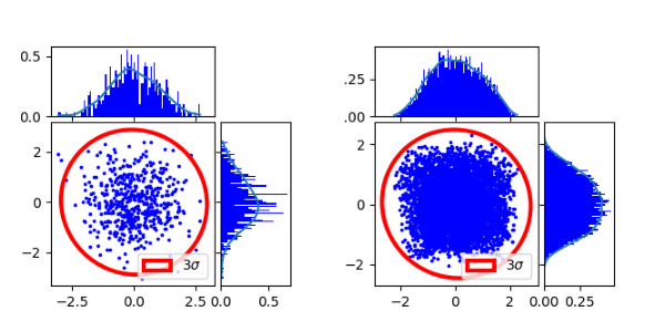
We plot the original distribution vs the generated one

params = display_historical_vs_generated_distribution(params)
params["graphic"](params)
plt.show()

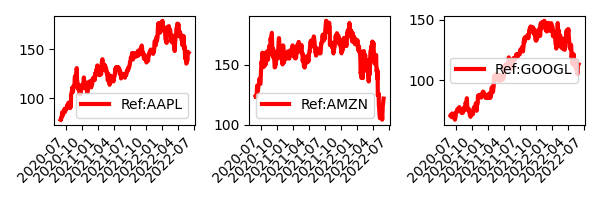
Reproductibility test

We regenerate the same path by generating from the latent representation We make sure we get the original data back.

params["reproductibility"] = True
params = generate_paths(params)
params["graphic"](params)
plt.show()

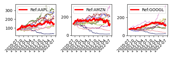
We now generate a new set of 10 paths

params["reproductibility"] = False
params["Nz"] = 10
params = generate_paths(params)
params["graphic"](params)
plt.show()
pass