3.4.1 Gradient Operator

This tutorial illustrates how to approximate gradients of a multivariate function using kernel-based operators provided by CodPy. It also introduces how the CodPy API implements these differential operators.

Overview

Given a positive-definite kernel function \(k\), CodPy defines a gradient operator \(\nabla_k\) over sets of input points \(X\):

\[ \nabla_k f_k(\cdot) = \nabla_k(\cdot) f(X), \quad \nabla_k(\cdot) = (\nabla K)(\cdot,X)( K(X,X) + \epsilon R(X,X) )^{-1} \]

where:

• \(X \in \mathbb{R}^{N_x \times D}\) is the training set,

• \(Y \in \mathbb{R}^{N_y \times D}\) is usually set equal to \(X\),

• \(Z \in \mathbb{R}^{N_z \times D}\) is the evaluation grid,

• \(K(X, Y)\) is the kernel Gram matrix of size \(\mathbb{R}^{N_x \times N_y}\),

• \(\nabla_k \in \mathbb{R}^{D \times N_z \times N_y}\) is the kernel gradient with respect to \(Z\).

This operator allows us to approximate the gradient of a function \(f\) evaluated at points \(Z\) using:

\[ \nabla_k f(Z) \approx \nabla_k(Z) \cdot f(X) \in \mathbb{R}^{D \times N_z \times D_f}, \]

where \(D_f\) is the output dimension of \(f\).

Map-Modified Gradient Operators

CodPy also supports applying maps \(S : \mathbb{R}^D \mapsto \mathbb{R}^D\) to transform the operator, resulting in:

\[ \nabla_{k \circ S}(Z) = (\nabla S)(Z) \cdot (\nabla_1 k)(\cdot,S(X))( K(S(X),S(X)) + \epsilon R(S(X),S(X)) )^{-1} \]

where:

• \((\nabla S)(Z) \in \mathbb{R}^{D \times D \times N_z}\) is the Jacobian of the map \(S\),

• \(( \nabla_1 k )\) refers to the gradient with respect to the first argument of \(k\).

Example with Periodic Function

We define a 2D periodic function \(f : \mathbb{R}^2 \mapsto \mathbb{R}\) as:

\[ f(\mathbf{x}) = \sum_{d=1}^2 x_d + \prod_{d=1}^2 \cos(2\pi x_d), \]

where \(\mathbf{x} = [x_1, x_2]^T\). This function is smooth and periodic in each input dimension. Its exact gradient is:

\[\begin{split} \nabla f(\mathbf{x}) = \begin{bmatrix} 1 - 2\pi \sin(2\pi x_1) \cos(2\pi x_2) \\ 1 - 2\pi \sin(2\pi x_2) \cos(2\pi x_1) \end{bmatrix} \end{split}\]

which is derived from the product rule applied to the cosine product term.

# to import necessary libraries
import os
import sys

from matplotlib import pyplot as plt

curr_f = os.path.join(os.getcwd(), "codpy-book", "utils")
sys.path.insert(0, curr_f)

import numpy as np

from codpy.plot_utils import multi_plot


# Define the sinusoidal function
def periodic_fun(x):
    """
    A sinusoidal function that generates a sum of sines based on the input ``x``.

    """
    from math import pi

    sinss = np.cos(2 * x * pi)
    if x.ndim == 1:
        sinss = np.prod(sinss, axis=0)
        ress = np.sum(x, axis=0)
    else:
        sinss = np.prod(sinss, axis=1)
        ress = np.sum(x, axis=1)
    return ress + sinss


def nabla_my_fun(x):
    from math import pi

    import numpy as np

    sinss = np.cos(2 * x * pi)
    if x.ndim == 1:
        sinss = np.prod(sinss, axis=0)
        D = len(x)
        out = np.ones((D))

        def helper(d):
            out[d] += 2.0 * sinss * pi * np.sin(2 * x[d] * pi) / np.cos(2 * x[d] * pi)

        [helper(d) for d in range(0, D)]
    else:
        sinss = np.prod(sinss, axis=1)
        N = x.shape[0]
        D = x.shape[1]
        out = np.ones((N, D))

        def helper(d):
            out[:, d] += (
                2.0 * sinss * pi * np.sin(2 * x[:, d] * pi) / np.cos(2 * x[:, d] * pi)
            )

        [helper(d) for d in range(0, D)]
    return out


# Function to generate periodic data
def generate_periodic_data_cartesian(size_x, size_z, fun=None, nabla_fun=None):
    """
    Generates 2D structured Cartesian grid data for x and z domains,
    and evaluates a given function and optionally its gradient.

    Parameters:
    - size_x: number of points per axis for x (grid will be size_x^2)
    - size_z: number of points per axis for z (grid will be size_z^2)
    - fun: function to evaluate at each point
    - nabla_fun: optional gradient function to evaluate

    Returns:
    - x, z: 2D Cartesian grids of shape (N, 2)
    - fx, fz: function values at x and z
    - nabla_fx, nabla_fz (if nabla_fun is provided)

    """

    def cartesian_grid(size, box):
        lin = [np.linspace(box[0, d], box[1, d], size) for d in range(2)]
        X, Y = np.meshgrid(*lin)
        return np.stack([X.ravel(), Y.ravel()], axis=1)

    # Define domain boxes
    X_box = np.array([[-1, -1], [1, 1]])
    Z_box = np.array([[-1.5, -1.5], [1.5, 1.5]])

    # Generate Cartesian grids
    x = cartesian_grid(size_x, X_box)
    z = cartesian_grid(size_z, Z_box)

    # Function evaluations
    fx = fun(x).reshape(-1, 1) if fun else None
    fz = fun(z).reshape(-1, 1) if fun else None

    if nabla_fun:
        nabla_fx = nabla_fun(x)
        nabla_fz = nabla_fun(z)
        return x, fx, z, fz, nabla_fx, nabla_fz

    return x, fx, z, fz


# Lets define helper function to plot 3D projection of the function
def plot_trisurf(xfx, ax, legend="", elev=90, azim=-100, **kwargs):
    from matplotlib import cm

    """
    Helper function to plot a 3D surface using a trisurf plot.

    Parameters:
    - xfx: A tuple containing the x-coordinates (2D points) and their
      corresponding function values.
    - ax: The matplotlib axis object for plotting.
    - legend: The legend/title for the plot.
    - elev, azim: Elevation and azimuth angles for the 3D view.
    - kwargs: Additional keyword arguments for further customization.

    """

    xp, fxp = xfx[0], xfx[1]
    x, fx = xp, fxp

    X, Y = x[:, 0], x[:, 1]
    Z = fx.flatten()
    ax.plot_trisurf(X, Y, Z, antialiased=False, cmap=cm.jet)
    ax.view_init(azim=azim, elev=elev)
    ax.title.set_text(legend)

CodPy Implementation using gradient operator

We use TensorNorm kernel function defined as:

\[ k(x, y) = \prod_{d} \max(1 - \|x_d - y_d\|, 0) \]

and the unit cube map \(S\):

\[ S(X) = \frac{x - \min_n{x^n} + \frac{0.5}{N_x}}{\alpha}, \quad \alpha = \max_n{x^n} - \min_n{x^n} \]

To compute the gradient of a function \(f(x)\) numerically using CodPy, we need: to import CodPy’s core module and Kernel class and initialize kernel pointer.

---

from codpy import core
from codpy.kernel import Kernel


def fun_nabla1(size_x=50, size_y=50):
    """

    Parameters:
    - data_x: List of generated x arrays.
    - data_fx: List of function values corresponding to each x.
    - data_z: List of generated z arrays.

    """
    # Apply CodPy and SciPy models for each (x, fx, z) pair

    x, fx, z, fz, _, nabla_fz = generate_periodic_data_cartesian(
        size_x, size_y, periodic_fun, nabla_fun=nabla_my_fun
    )

    nabla_fz = nabla_fz.reshape(-1, 2, 1)

    nabla_f_x = Kernel(
            x=x, fx=fx, set_kernel=core.kernel_setter("gaussianper", None,2, 1e-8),order=2,reg=1e-8
        ).grad(z)

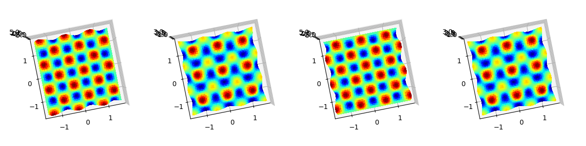
    multi_plot(
        [
            (z, nabla_fz[:, 0, :]),
            (z, nabla_f_x[:, 0, :]),
            (z, nabla_fz[:, 1, :]),
            (z, nabla_f_x[:, 1, :]),
        ],
        plot_trisurf,
        projection="3d",
        mp_max_items=4,
        mp_ncols=4,
        mp_nrows=1,
        mp_figsize=(12, 3),
    )
    plt.show()


fun_nabla1()

CodPy Implementation using Kernel class

To compute the gradient of a function \(f(x)\) numerically using CodPy, we need: to import CodPy’s core module and Kernel class and initialize kernel pointer:

---

def fun_nabla2(size_x=50, size_y=50):
    """

    Parameters:
    - data_x: List of generated x arrays.
    - data_fx: List of function values corresponding to each x.
    - data_z: List of generated z arrays.

    """
    # Apply CodPy and SciPy models for each (x, fx, z) pair

    x, fx, z, fz, _, nabla_fz = generate_periodic_data_cartesian(
        size_x, size_y, periodic_fun, nabla_fun=nabla_my_fun
    )

    nabla_fz = nabla_fz.reshape(-1, 2, 1)
    kernel = Kernel(
        set_kernel=core.kernel_setter("gaussianper", None,2, 1e-8),
        x=x,
        fx=fx,
        y=x,
        order=2,
        reg=1e-8,
    )
    nabla_f_x = kernel.grad(z)

    multi_plot(
        [
            (z, nabla_fz[:, 0, :]),
            (z, nabla_f_x[:, 0, :]),
            (z, nabla_fz[:, 1, :]),
            (z, nabla_f_x[:, 1, :]),
        ],
        plot_trisurf,
        projection="3d",
        mp_max_items=4,
        mp_ncols=4,
        mp_nrows=1,
        mp_figsize=(12, 3),
    )
    plt.show()


fun_nabla2()
pass