7.03 Heat Equation

We reproduce here the figure 7.4 & 7.5 of the book. Utilitary functions can be found next to this file. Here, we only define codpy-related functions.

Necessary Imports

import os
import sys

import matplotlib.pyplot as plt

try:
    CURRENT_DIR = os.path.dirname(os.path.abspath(__file__))
except NameError:
    CURRENT_DIR = os.getcwd()
data_path = os.path.join(CURRENT_DIR, "data")
PARENT_DIR = os.path.abspath(os.path.join(CURRENT_DIR, ".."))
sys.path.insert(0, PARENT_DIR)

from utils.ch7.ch7_utils import PDE3, PDE4

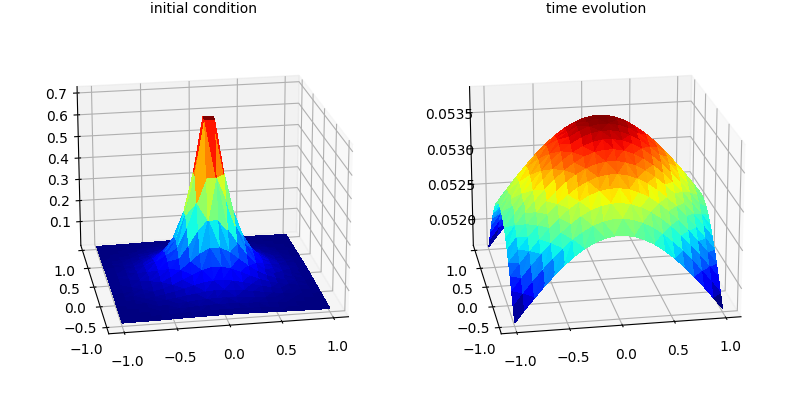
Problem statement

let’s consider the heat equation in a fixed geometry \(\Omega\) with null Dirichlet conditions:

\[\partial_t u(t,x) = \Delta u(t,x), \quad u(0,x)=u_0(x),\quad x \in \Omega, \quad u_{\partial \Omega}=0\]

To approximate this equation, we follow the following steps: Select a mesh \(X \in \mathbb{R}^{N_x,D}\) for the domain \(\Omega\). Pick up a kernel \(k\) generating a space of vanishing trace functions. We represent this equation as \(\frac{d}{dt} u(t) = \Delta_k u(t)\), with evolution operator \(u^{n+1} = B(\Delta_k,u^{n},dt,\theta)\) and \(\theta = 1\). This corresponds to the fully implicit case

Regular mesh

This image provides a 3-D representation of the initial condition and time evolution of the heat equation on a fixed square.

PDE3()
plt.show()

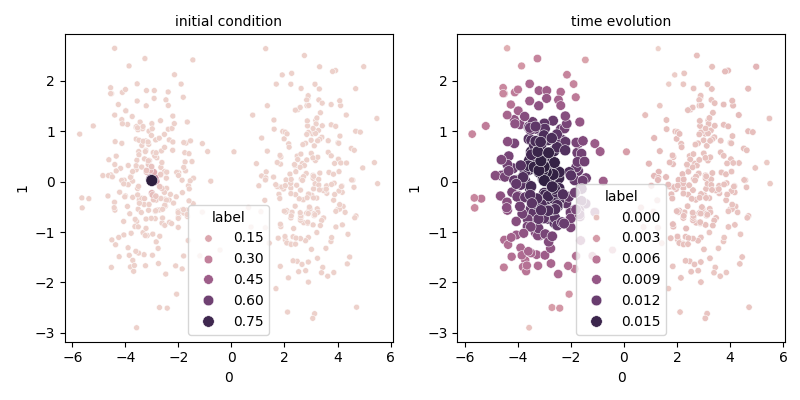
Irregular mesh

This image shows the heat equation on an irregular mesh generated by a bimodal Gaussian process.

PDE4()
plt.show()
pass