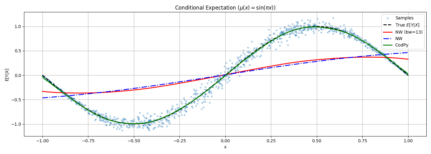
5.3.4 Kernel Conditional Expectation

We benchmark the performance of different conditional density estimators: - Nadaraya–Watson (standard with bw = 13) - Nadaraya–Watson with mean scaled Matern kernel - CodPy’s projection-based ConditionerKernel

We generate synthetic data with a nonlinear conditional mean and heteroscedastic variance.

Mathematically, the data is generated as:

\[ X \sim \mathcal{U}(-1, 1), \quad Y \mid X = x \sim \mathcal{N}\big( \mu(x), \sigma^2(x) \big) \]

where:

• Conditional mean: \(\mu(x) = \cos(2\pi x)\)

• Conditional standard deviation: \(\sigma(x) = 0.1 \cdot \cos\left( \frac{\pi x}{2} \right)\)

This allows us to test both the ability to recover nonlinear trends in the conditional mean and to handle non-constant conditional variance.

We compare estimated conditional expectations \(\mathbb{E}[Y \mid X=x]\) with the ground truth \(\mu(x)\) across a grid of evaluation points.

Required imports

import matplotlib.pyplot as plt
import numpy as np
from scipy.stats import norm

from codpy.conditioning import ConditionerKernel, NadarayaWatsonKernel
from codpy.core import kernel_setter
import codpy.core

codpy.core.KerInterface.set_verbose()

Generating the data

The data is generated according to the chapter 5.3.3 of the book. - Illustrative example.

def mean_function_hard(x):
    return np.cos(2 * np.pi * x)


def variance_function(x):
    return 0.1 * np.cos(np.pi * x * 0.5)


def mean_function(x):
    return np.sin(np.pi * x)


def variance_function_hard(X):
    return 0.3 - 0.1 * mean_function(X)


def generate_conditional_hetero_skedastic_density_data(
    N_train=1000, seed=None, mean_f=None, variance_f=None
):
    """
    Generate synthetic data with nonlinear and heteroscedastic structure.

    Parameters:
    - N_train: Number of training samples (X, Y)
    - seed: Random seed for reproducibility
    - mean_f: Callable for mean function, e.g., mean_function(x)
    - variance_f: Callable for variance function, e.g., variance_function(x)

    Returns:
    - x: Training input samples (1D array)
    - y: Training output samples (1D array)
    - z: Test input sample (scalar)
    - y_pdf: Grid of y values for PDF estimation
    - (fz_mean, fz_std): True conditional mean and std at z
    - density: True conditional density at z over y_pdf
    """
    if seed is not None:
        np.random.seed(seed)

    if mean_f is None:
        mean_f = mean_function
    if variance_f is None:
        variance_f = variance_function

    x = np.random.uniform(-1.0, 1.0, N_train)

    mean_y = mean_f(x)
    std_y = variance_f(x)

    y = np.random.normal(loc=mean_y, scale=std_y)

    z = 0.0
    fz_mean = mean_f(z)
    fz_std = variance_f(z)

    y_pdf = np.linspace(2.0 * y.min(), 2.0 * y.max(), N_train)
    density = norm.pdf(y_pdf, loc=fz_mean, scale=fz_std)
    density /= density.sum(axis=0)

    return x, y, z, y_pdf, (fz_mean, fz_std), density

Full curve: conditional mean across a grid

fig, axes = plt.subplots(1, 1, figsize=(14, 5))
X_eval = np.linspace(-1, 1, 300)

# Case 1 (Smooth, theta = \pi/2)
x, y, z, y_pdf, (fz_mean, fz_std), density = (
    generate_conditional_hetero_skedastic_density_data(
        N_train=1000,
        seed=3,
        mean_f=mean_function,
        variance_f=variance_function,
    )
)
Y_true_easy = mean_function(X_eval)

# Estimators
nw_model_easy = NadarayaWatsonKernel(x=x, y=y)
Y_nw_easy = nw_model_easy.expectation(X_eval)

kde_model_easy = NadarayaWatsonKernel(
    x=x,
    y=y,
    set_kernel=kernel_setter(kernel_string="gaussian",map_args= {"bandwidth": 13}),
)
Y_kde_easy = kde_model_easy.expectation(X_eval)

codpy_model_easy = ConditionerKernel(x=x, y=y)
Y_codpy_easy = codpy_model_easy.expectation(X_eval, reg=100)

plt.scatter(x, y, alpha=0.3, s=10, label="Samples")
plt.plot(X_eval, Y_true_easy, "k--", lw=2, label="True $E[Y|X]$")
plt.plot(X_eval, Y_nw_easy, "r-", lw=2, label="NW (bw=13)")
plt.plot(X_eval, Y_kde_easy, "b-.", lw=2, label="NW")
plt.plot(X_eval, Y_codpy_easy, "g", lw=2, label="CodPy")
plt.title(r"Conditional Expectation ($\mu(x) = \sin(\pi x)$)")
plt.xlabel("x")
plt.ylabel("E[Y|X]")
plt.legend()
plt.grid(True)
plt.tight_layout()
plt.show()