3.3.2 Partition of unity

This section introduces the concept of partition of unity in the context of kernel methods and how CodPy implements it via projection operators.

Overview

Given a positive-definite kernel function \(k\) and a set of input points \(X \in \mathbb{R}^{N_x \times D}\), CodPy defines a projection operator based on the kernel Gram matrix. This leads to a kernel-based partition of unity function defined over a set of evaluation points \(Y \in \mathbb{R}^{N_y \times D}\).

The partition of unity function \(\phi\) is defined as:

\[ \phi(Y) = K(Y, X) K(X, X)^{-1} \in \mathbb{R}^{N_y \times N_x}, \]

where:

• \(K(Y, X)\) is the kernel Gram matrix between \(Y\) and \(X\),

• \(K(X, X)\) is the self-Gram matrix of the training set \(X\),

• \(\phi^m(Y)\) denotes the \(m\)-th component function of the partition.

This operator assigns to each point \(y \in Y\) a set of weights \((\phi^1(y), \ldots, \phi^{N_x}(y))\) corresponding to its projection onto the basis functions centered at points in \(X\).

Delta Property

A key feature of this partition is that it interpolates exactly at the input points \(x^n \in X\). That is, for all \(x^n \in X\):

\[ \phi(x^n) = (0, \ldots, 1, \ldots, 0) = \delta_{n,m}, \]

where \(\delta_{n,m}\) is the Kronecker delta symbol, equal to \(1\) if \(n = m\) and \(0\) otherwise. This ensures the projection perfectly reconstructs function values at the training inputs.

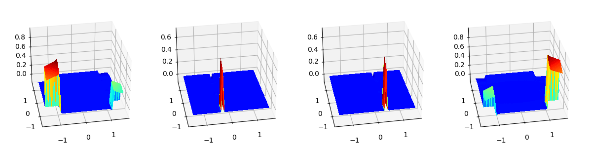
Figure illustrates the concept with an example involving four basis points \(X = \{x^1, x^2, x^3, x^4\}\) and shows the corresponding four partition functions \(\phi^1(Y), \ldots, \phi^4(Y)\). Each function is peaked at its associated center and decays smoothly, yet together they form a partition of unity over the domain.

# Importing necessary modules
import os
import sys

from matplotlib import pyplot as plt

curr_f = os.path.join(os.getcwd(), "codpy-book", "utils")
sys.path.insert(0, curr_f)


import numpy as np

# from codpy.plotting import plot1D
# Lets import multi_plot function from codpy utils
from codpy.plot_utils import multi_plot


# Define the sinusoidal function
def periodic_fun(x):
    """
    A sinusoidal function that generates a sum of sines based on the input ``x``.
    """
    from math import pi

    sinss = np.cos(2 * x * pi)
    if x.ndim == 1:
        sinss = np.prod(sinss, axis=0)
        ress = np.sum(x, axis=0)
    else:
        sinss = np.prod(sinss, axis=1)
        ress = np.sum(x, axis=1)
    return ress + sinss


# Function to generate periodic data
def generate_periodic_data_cartesian(size_x, size_z, fun=None, nabla_fun=None):
    """
    Generates 2D structured Cartesian grid data for x and z domains,
    and evaluates a given function and optionally its gradient.

    Parameters:
    - size_x: number of points per axis for x (grid will be size_x^2)
    - size_z: number of points per axis for z (grid will be size_z^2)
    - fun: function to evaluate at each point
    - nabla_fun: optional gradient function to evaluate

    Returns:
    - x, z: 2D Cartesian grids of shape (N, 2)
    - fx, fz: function values at x and z
    - nabla_fx, nabla_fz (if nabla_fun is provided)
    """

    def cartesian_grid(size, box):
        lin = [np.linspace(box[0, d], box[1, d], size) for d in range(2)]
        X, Y = np.meshgrid(*lin)
        return np.stack([X.ravel(), Y.ravel()], axis=1)

    # Define domain boxes
    X_box = np.array([[-1, -1], [1, 1]])
    Z_box = np.array([[-1.5, -1.5], [1.5, 1.5]])

    # Generate Cartesian grids
    x = cartesian_grid(size_x, X_box)
    z = cartesian_grid(size_z, Z_box)

    # Function evaluations
    fx = fun(x).reshape(-1, 1) if fun else None
    fz = fun(z).reshape(-1, 1) if fun else None

    if nabla_fun:
        nabla_fx = nabla_fun(x)
        nabla_fz = nabla_fun(z)
        return x, z, fx, fz, nabla_fx, nabla_fz

    return x, fx, z, fz


# Lets define helper function to plot 3D projection of the function
def plot_trisurf(xfx, ax, legend="", elev=90, azim=-100, **kwargs):
    from matplotlib import cm

    """
    Helper function to plot a 3D surface using a trisurf plot.

    Parameters:
    - xfx: A tuple containing the x-coordinates (2D points) and their
      corresponding function values.
    - ax: The matplotlib axis object for plotting.
    - legend: The legend/title for the plot.
    - elev, azim: Elevation and azimuth angles for the 3D view.
    - kwargs: Additional keyword arguments for further customization.
    """

    xp, fxp = xfx[0], xfx[1]
    x, fx = xp, fxp

    X, Y = x[:, 0], x[:, 1]
    Z = fx.flatten()
    ax.plot_trisurf(X, Y, Z, antialiased=False, cmap=cm.jet)
    ax.view_init(azim=azim, elev=elev)
    ax.title.set_text(legend)


# import CodPy's core module and Kernel class
from codpy import core
from codpy.kernel import Kernel


def fun_part():
    """
    Runs the experiment applying CodPy and SciPy models on the data and plots the results.

    Parameters:
    - data_x: List of generated x arrays.
    - data_fx: List of function values corresponding to each x.
    - data_z: List of generated z arrays.
    """
    # Apply CodPy and SciPy models for each (x, fx, z) pair

    x, fx, z, fz = generate_periodic_data_cartesian(50, 50)

    kernel = Kernel(
        set_kernel=core.kernel_setter("tensornorm", "scale_to_unitcube"),
        x=x,
        y=x,
        order=2,
        reg=1e-8,
    )
    partxxz = kernel(z).T
    temp = int(np.sqrt(z.shape[0]))

    multi_plot(
        [(z, partxxz[0, :]), (z, partxxz[int(temp / 3), :])]
        + [(z, partxxz[int(temp * 2 / 3), :]), (z, partxxz[temp - 1, :])],
        plot_trisurf,
        projection="3d",
        elev=30,
        mp_nrows=1,
        mp_figsize=(12, 3),
    )
    plt.show()


fun_part()