7.01 Inverse Laplace Operator

We reproduce here the figure 7.1 and 7.2 of the book. Utilitary functions can be found next to this file. Here, we only define codpy-related functions.

Necessary Imports

import os
import sys

import matplotlib.pyplot as plt
from codpy import core

try:
    CURRENT_DIR = os.path.dirname(os.path.abspath(__file__))
except NameError:
    CURRENT_DIR = os.getcwd()
data_path = os.path.join(CURRENT_DIR, "data")
PARENT_DIR = os.path.abspath(os.path.join(CURRENT_DIR, ".."))
sys.path.insert(0, PARENT_DIR)

from utils.ch7.ch7_utils import PDE1, PDE2

Problem statement

We solve the following Poisson equation with Dirichlet boundary conditions:

\[\Delta u = f, \quad \text{ supp } u \subset \Omega, \quad u_{\partial \Omega}=0\]

where \(f\) is sufficient regular and \(\Omega\) is a sufficient regular domain. To do so we select a mesh, and a kernel, which approximates this equation by approximating the solution as a function \(u \in \mathcal{H}_k\) This leads to the equation \((\Delta_k u)(X) = f(X)\), \(\Delta_k\) being the approximation of the Laplace-Beltrami operator defined in the book. A solution to this equation is computed as \(u = (\Delta_k)^{-1} f\).

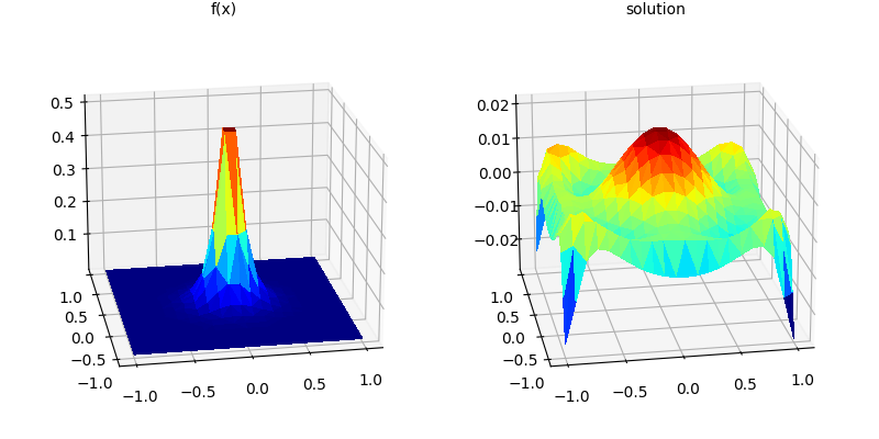
Regular mesh

This figure displays a regular mesh for the domain \(\Omega = [0,1]^2\), where \(f\) is plotted in the left-hand side, and the solution \(u\) in the right-hand side.

PDE1()
plt.show()

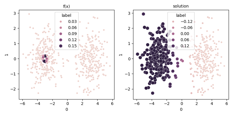
Irregular mesh

This figure computes a Poisson equation on an unstructured mesh generated by a bimodal Gaussian random variable, with \(f\) plotted on the left and the solution \(u\) on the right.

PDE2()
plt.show()